The Shapely User Manual#
- Author:
Sean Gillies, <sean.gillies@gmail.com>
- Version:
2.1.1
- Date:
Jul 07, 2026
- Copyright:
This work is licensed under a Creative Commons Attribution 3.0 United States License.
- Abstract:
This document explains how to use the Shapely Python package for computational geometry.
Introduction#
Deterministic spatial analysis is an important component of computational approaches to problems in agriculture, ecology, epidemiology, sociology, and many other fields. What is the surveyed perimeter/area ratio of these patches of animal habitat? Which properties in this town intersect with the 50-year flood contour from this new flooding model? What are the extents of findspots for ancient ceramic wares with maker’s marks “A” and “B”, and where do the extents overlap? What’s the path from home to office that best skirts identified zones of location based spam? These are just a few of the possible questions addressable using non-statistical spatial analysis, and more specifically, computational geometry.
Shapely is a Python package for set-theoretic analysis and manipulation of planar features using functions from the well known and widely deployed GEOS library. GEOS, a port of the Java Topology Suite (JTS), is the geometry engine of the PostGIS spatial extension for the PostgreSQL RDBMS. The designs of JTS and GEOS are largely guided by the Open Geospatial Consortium’s Simple Features Access Specification [1] and Shapely adheres mainly to the same set of standard classes and operations. Shapely is thereby deeply rooted in the conventions of the geographic information systems (GIS) world, but aspires to be equally useful to programmers working on non-conventional problems.
The first premise of Shapely is that Python programmers should be able to perform PostGIS type geometry operations outside of an RDBMS. Not all geographic data originate or reside in a RDBMS or are best processed using SQL. We can load data into a spatial RDBMS to do work, but if there’s no mandate to manage (the “M” in “RDBMS”) the data over time in the database we’re using the wrong tool for the job. The second premise is that the persistence, serialization, and map projection of features are significant, but orthogonal problems. You may not need a hundred GIS format readers and writers or the multitude of State Plane projections, and Shapely doesn’t burden you with them. The third premise is that Python idioms trump GIS (or Java, in this case, since the GEOS library is derived from JTS, a Java project) idioms.
If you enjoy and profit from idiomatic Python, appreciate packages that do one thing well, and agree that a spatially enabled RDBMS is often enough the wrong tool for your computational geometry job, Shapely might be for you.
Spatial Data Model#
The fundamental types of geometric objects implemented by Shapely are points, curves, and surfaces. Each is associated with three sets of (possibly infinite) points in the plane. The interior, boundary, and exterior sets of a feature are mutually exclusive and their union coincides with the entire plane [2].
A Point has an interior set of exactly one point, a boundary set of exactly no points, and an exterior set of all other points. A Point has a topological dimension of 0.
A Curve has an interior set consisting of the infinitely many points along its length (imagine a Point dragged in space), a boundary set consisting of its two end points, and an exterior set of all other points. A Curve has a topological dimension of 1.
A Surface has an interior set consisting of the infinitely many points within (imagine a Curve dragged in space to cover an area), a boundary set consisting of one or more Curves, and an exterior set of all other points including those within holes that might exist in the surface. A Surface has a topological dimension of 2.
That may seem a bit esoteric, but will help clarify the meanings of Shapely’s spatial predicates, and it’s as deep into theory as this manual will go. Consequences of point-set theory, including some that manifest themselves as “gotchas”, for different classes will be discussed later in this manual.
The point type is implemented by a Point class; curve by the LineString and LinearRing classes; and surface by a Polygon class. Shapely implements no smooth (i.e. having continuous tangents) curves. All curves must be approximated by linear splines. All rounded patches must be approximated by regions bounded by linear splines.
Collections of points are implemented by a MultiPoint class, collections of curves by a MultiLineString class, and collections of surfaces by a MultiPolygon class. These collections aren’t computationally significant, but are useful for modeling certain kinds of features. A Y-shaped line feature, for example, is well modeled as a whole by a MultiLineString.
The standard data model has additional constraints specific to certain types of geometric objects that will be discussed in following sections of this manual.
See also https://web.archive.org/web/20160719195511/http://www.vividsolutions.com/jts/discussion.htm for more illustrations of this data model.
Relationships#
The spatial data model is accompanied by a group of natural language relationships between geometric objects – contains, intersects, overlaps, touches, etc. – and a theoretical framework for understanding them using the 3x3 matrix of the mutual intersections of their component point sets [3]: the DE-9IM. A comprehensive review of the relationships in terms of the DE-9IM is found in [4] and will not be reiterated in this manual.
Operations#
Following the JTS technical specs [5], this manual will make a distinction between constructive (buffer, convex hull) and set-theoretic operations (intersection, union, etc.). The individual operations will be fully described in a following section of the manual.
Coordinate Systems#
Even though the Earth is not flat – and for that matter not exactly spherical – there are many analytic problems that can be approached by transforming Earth features to a Cartesian plane, applying tried and true algorithms, and then transforming the results back to geographic coordinates. This practice is as old as the tradition of accurate paper maps.
Shapely does not support coordinate system transformations. All operations on two or more features presume that the features exist in the same Cartesian plane.
Geometric Objects#
Geometric objects are created in the typical Python fashion, using the classes themselves as instance factories. A few of their intrinsic properties will be discussed in this sections, others in the following sections on operations and serializations.
Instances of Point, LineString, and LinearRing have as their most
important attribute a finite sequence of coordinates that determines their
interior, boundary, and exterior point sets. A line string can be determined by
as few as 2 points, but contains an infinite number of points. Coordinate
sequences are immutable. A third z coordinate value may be used when
constructing instances, but has no effect on geometric analysis. All
operations are performed in the x-y plane.
In all constructors, numeric values are converted to type float. In other
words, Point(0, 0) and Point(0.0, 0.0) produce geometrically equivalent
instances. Shapely does not check the topological simplicity or validity of
instances when they are constructed as the cost is unwarranted in most cases.
Validating factories are easily implemented using the :attr:is_valid
predicate by users that require them.
Note
Shapely is a planar geometry library and z, the height
above or below the plane, is ignored in geometric analysis. There is
a potential pitfall for users here: coordinate tuples that differ only in
z are not distinguished from each other and their application can result
in surprisingly invalid geometry objects. For example, LineString([(0, 0,
0), (0, 0, 1)]) does not return a vertical line of unit length, but an invalid line
in the plane with zero length. Similarly, Polygon([(0, 0, 0), (0, 0, 1),
(1, 1, 1)]) is not bounded by a closed ring and is invalid.
General Attributes and Methods#
- object.area#
Returns the area (
float) of the object.
- object.bounds#
Returns a
(minx, miny, maxx, maxy)tuple (floatvalues) that bounds the object.
- object.length#
Returns the length (
float) of the object.
- object.minimum_clearance#
Returns the smallest distance by which a node could be moved to produce an invalid geometry.
This can be thought of as a measure of the robustness of a geometry, where larger values of minimum clearance indicate a more robust geometry. If no minimum clearance exists for a geometry, such as a point, this will return math.infinity.
New in Shapely 1.7.1
>>> from shapely import Polygon
>>> Polygon([[0, 0], [1, 0], [1, 1], [0, 1], [0, 0]]).minimum_clearance
1.0
- object.geom_type#
Returns a string specifying the Geometry Type of the object in accordance with [1].
>>> from shapely import Point, LineString
>>> Point(0, 0).geom_type
'Point'
- object.distance(other)#
Returns the minimum distance (
float) to the other geometric object.
>>> Point(0,0).distance(Point(1,1))
1.4142135623730951
- object.hausdorff_distance(other)#
Returns the Hausdorff distance (
float) to the other geometric object.Check out
shapely.hausdorff_distance()for more details.New in Shapely 1.6.0
>>> point = Point(1, 1)
>>> line = LineString([(2, 0), (2, 4), (3, 4)])
>>> point.hausdorff_distance(line)
3.605551275463989
>>> point.distance(Point(3, 4))
3.605551275463989
- object.representative_point()#
Returns a cheaply computed point that is guaranteed to be within the geometric object.
Note
This is not in general the same as the centroid.
>>> diamond = Point(0, 0).buffer(2.0, 1).difference(Point(0, 0).buffer(1.0, 1))
>>> diamond.centroid
<POINT (0 0)>
>>> diamond.representative_point()
<POINT (-1 0.5)>
Points#
- class Point(coordinates)#
The Point constructor takes positional coordinate values or point tuple parameters.
>>> from shapely import Point
>>> point = Point(0.0, 0.0)
>>> q = Point((0.0, 0.0))
A Point has zero area and zero length.
>>> point.area
0.0
>>> point.length
0.0
Its x-y bounding box is a (minx, miny, maxx, maxy) tuple.
>>> point.bounds
(0.0, 0.0, 0.0, 0.0)
Coordinate values are accessed via coords, x, y, z, and m properties.
>>> list(point.coords)
[(0.0, 0.0)]
>>> point.x
0.0
>>> point.y
0.0
Coordinates may also be sliced. New in version 1.2.14.
>>> point.coords[:]
[(0.0, 0.0)]
When a Point instance is passed to the Point constructor, it returns a reference to the passed instance. It does not make a copy, as geometry objects are immutable.
>>> Point(point)
<POINT (0 0)>
LineStrings#
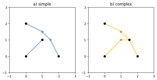
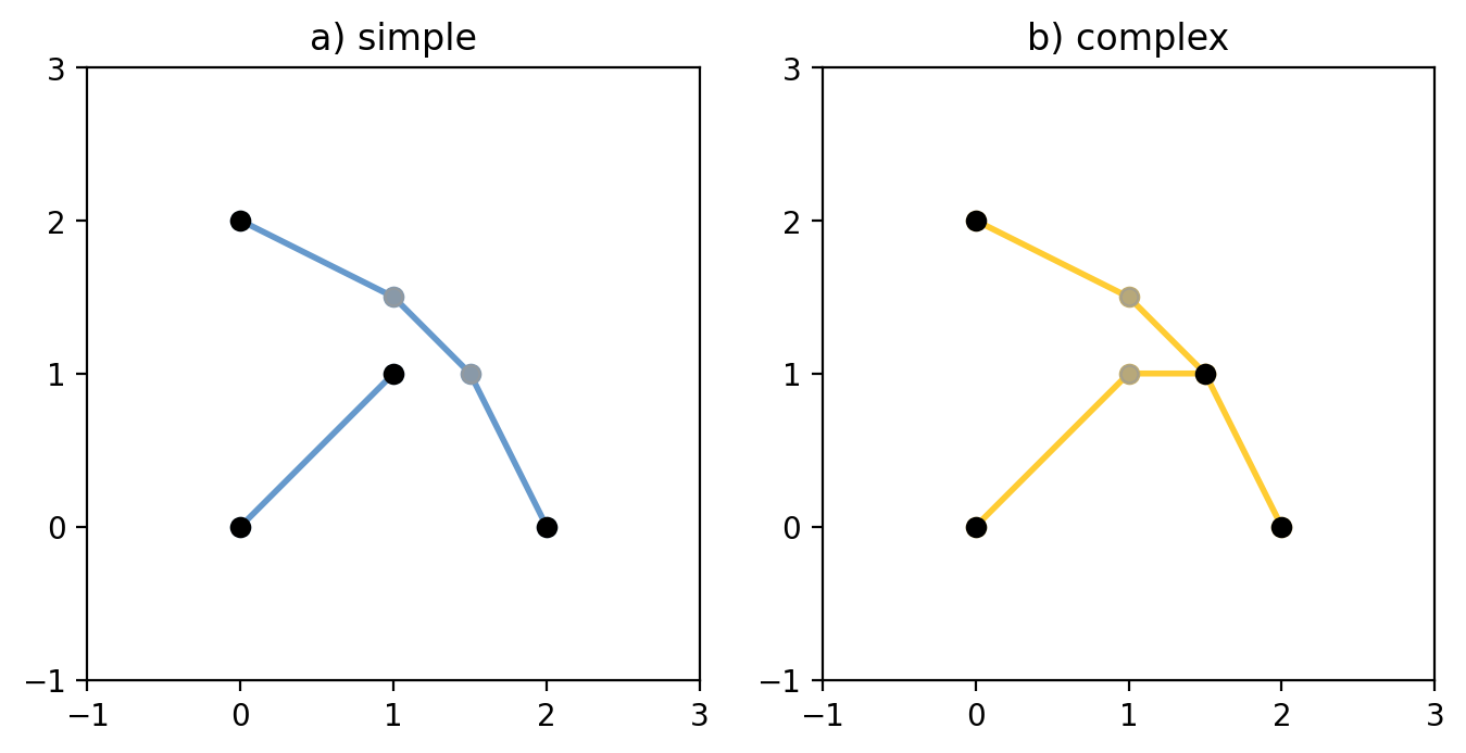
- class LineString(coordinates)#
The LineString constructor takes an ordered sequence of 2 or more
(x, y[, z])point tuples.
The constructed LineString object represents one or more connected linear splines between the points. Repeated points in the ordered sequence are allowed, but may incur performance penalties and should be avoided. A LineString may cross itself (i.e. be complex and not simple).
(Source code, png, hires.png, pdf)
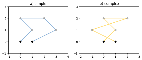
Figure 1. A simple LineString on the left, a complex LineString on the right. The (MultiPoint) boundary of each is shown in black, the other points that describe the lines are shown in grey.
A LineString has zero area and non-zero length if it isn’t empty.
>>> from shapely import LineString
>>> line = LineString([(0, 0), (1, 1)])
>>> line.area
0.0
>>> line.length
1.4142135623730951
Its x-y bounding box is a (minx, miny, maxx, maxy) tuple.
>>> line.bounds
(0.0, 0.0, 1.0, 1.0)
The defining coordinate values are accessed via the coords property.
>>> len(line.coords)
2
>>> list(line.coords)
[(0.0, 0.0), (1.0, 1.0)]
Coordinates may also be sliced. New in version 1.2.14.
>>> line.coords[:]
[(0.0, 0.0), (1.0, 1.0)]
>>> line.coords[1:]
[(1.0, 1.0)]
When the constructor is passed another LineString instance, a reference to the instance is returned.
>>> LineString(line)
<LINESTRING (0 0, 1 1)>
A LineString may also be constructed using a sequence of mixed Point instances or coordinate tuples. The individual coordinates are copied into the new object.
>>> LineString([Point(0.0, 1.0), (2.0, 3.0), Point(4.0, 5.0)])
<LINESTRING (0 1, 2 3, 4 5)>
LinearRings#
- class LinearRing(coordinates)#
The LinearRing constructor takes an ordered sequence of
(x, y[, z])point tuples.
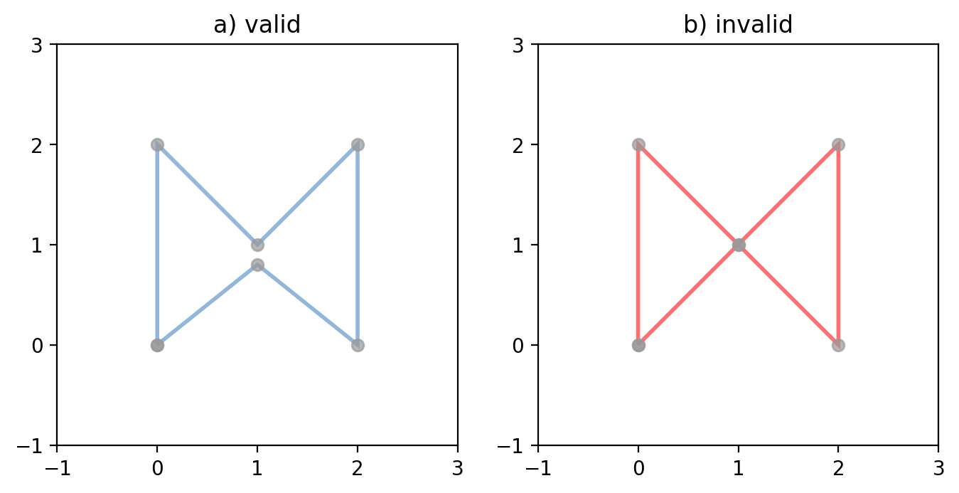
The sequence may be explicitly closed by passing identical values in the first and last indices. Otherwise, the sequence will be implicitly closed by copying the first tuple to the last index. As with a LineString, repeated points in the ordered sequence are allowed, but may incur performance penalties and should be avoided. A LinearRing may not cross itself, and may not touch itself at a single point.
(Source code, png, hires.png, pdf)
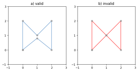
Figure 2. A valid LinearRing on the left, an invalid self-touching LinearRing on the right. The points that describe the rings are shown in grey. A ring’s boundary is empty.
Note
Shapely will not prevent the creation of such rings, but exceptions will be raised when they are operated on.
A LinearRing has zero area and non-zero length if it isn’t empty.
>>> from shapely import LinearRing
>>> ring = LinearRing([(0, 0), (1, 1), (1, 0)])
>>> ring.area
0.0
>>> ring.length
3.414213562373095
Its x-y bounding box is a (minx, miny, maxx, maxy) tuple.
>>> ring.bounds
(0.0, 0.0, 1.0, 1.0)
Defining coordinate values are accessed via the coords property.
>>> len(ring.coords)
4
>>> list(ring.coords)
[(0.0, 0.0), (1.0, 1.0), (1.0, 0.0), (0.0, 0.0)]
The LinearRing constructor also accepts another LineString or LinearRing instance, returning a new LinearRing instance or a reference to the passed instance, respectively.
>>> LinearRing(ring)
<LINEARRING (0 0, 1 1, 1 0, 0 0)>
As with LineString, a sequence of Point instances is a valid constructor parameter.
Polygons#
- class Polygon(shell[, holes=None])#
The Polygon constructor takes two positional parameters. The first is an ordered sequence of
(x, y[, z])point tuples and is treated exactly as in the LinearRing case. The second is an optional unordered sequence of ring-like sequences specifying the interior boundaries or “holes” of the feature.
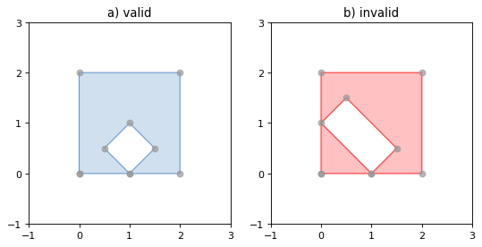
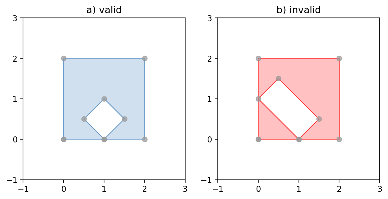
Rings of a valid Polygon may not cross each other, but may touch at a single point only. Again, Shapely will not prevent the creation of invalid features, but when they are operated on the results might be wrong or exceptions might be raised.
(Source code, png, hires.png, pdf)

Figure 3. On the left, a valid Polygon with one interior ring that touches the exterior ring at one point, and on the right a Polygon that is invalid because its interior ring touches the exterior ring at more than one point. The points that describe the rings are shown in grey.
(Source code, png, hires.png, pdf)
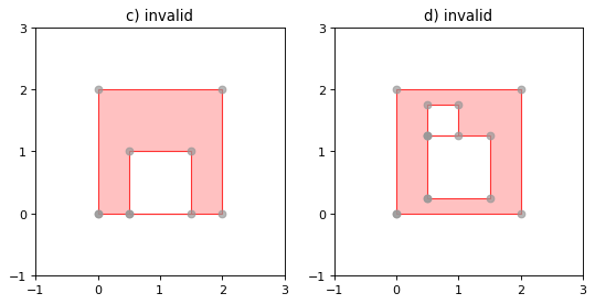
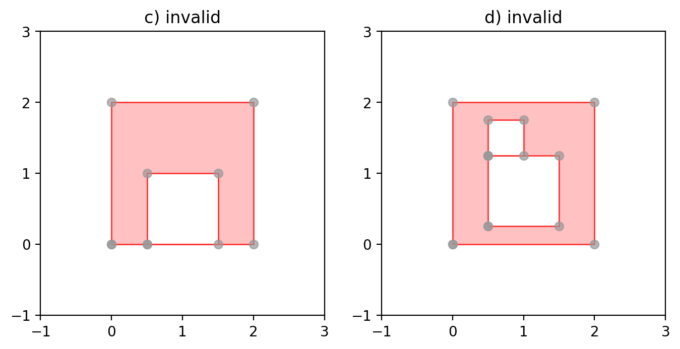
Figure 4. On the left, a Polygon that is invalid because its exterior and interior rings touch along a line, and on the right, a Polygon that is invalid because its interior rings touch along a line.
A Polygon has non-zero area and non-zero length if it isn’t empty.
>>> from shapely import Polygon
>>> polygon = Polygon([(0, 0), (1, 1), (1, 0)])
>>> polygon.area
0.5
>>> polygon.length
3.414213562373095
Its x-y bounding box is a (minx, miny, maxx, maxy) tuple.
>>> polygon.bounds
(0.0, 0.0, 1.0, 1.0)
Component rings are accessed via exterior and interiors properties.
>>> list(polygon.exterior.coords)
[(0.0, 0.0), (1.0, 1.0), (1.0, 0.0), (0.0, 0.0)]
>>> list(polygon.interiors)
[]
The Polygon constructor also accepts instances of LineString and LinearRing.
>>> coords = [(0, 0), (1, 1), (1, 0)]
>>> r = LinearRing(coords)
>>> s = Polygon(r)
>>> s.area
0.5
>>> t = Polygon(s.buffer(1.0).exterior, [r])
>>> t.area
6.5507620529190325
Rectangular polygons occur commonly, and can be conveniently constructed using
the shapely.geometry.box() function.
- shapely.geometry.box(minx, miny, maxx, maxy, ccw=True)#
Makes a rectangular polygon from the provided bounding box values, with counter-clockwise order by default.
New in version 1.2.9.
For example:
>>> from shapely import box
>>> b = box(0.0, 0.0, 1.0, 1.0)
>>> b
<POLYGON ((1 0, 1 1, 0 1, 0 0, 1 0))>
>>> list(b.exterior.coords)
[(1.0, 0.0), (1.0, 1.0), (0.0, 1.0), (0.0, 0.0), (1.0, 0.0)]
This is the first appearance of an explicit polygon handedness in Shapely.
To obtain a polygon with a known orientation, use
shapely.geometry.polygon.orient():
- shapely.geometry.polygon.orient(polygon, sign=1.0)#
Returns a new Polygon instance with the coordinates of the given polygon in proper orientation. The signed area of the result will have the given sign. A sign of 1.0 means that the coordinates of the product’s exterior ring will be oriented counter-clockwise and the interior rings (holes) will be oriented clockwise.
New in version 1.2.10.
Collections#
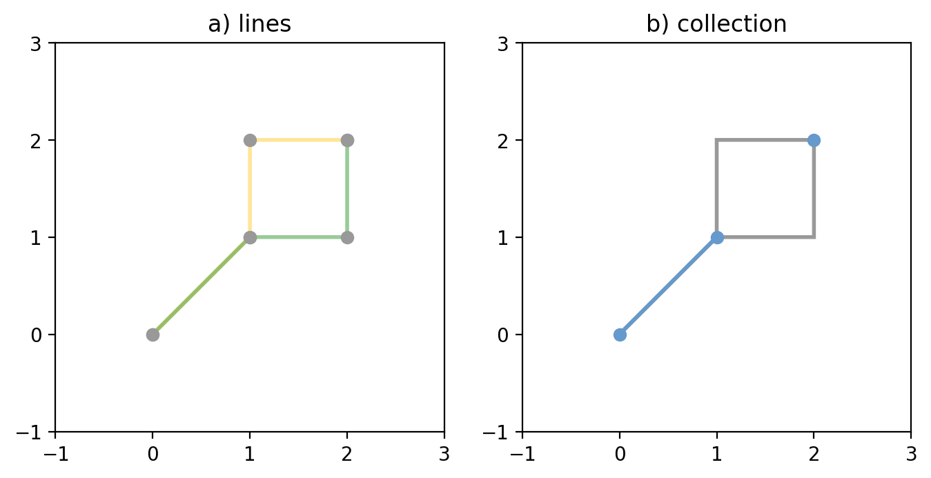
Heterogeneous collections of geometric objects may result from some Shapely operations. For example, two LineStrings may intersect along a line and at a point. To represent these kind of results, Shapely provides frozenset-like, immutable collections of geometric objects. The collections may be homogeneous (MultiPoint etc.) or heterogeneous.
>>> a = LineString([(0, 0), (1, 1), (1,2), (2,2)])
>>> b = LineString([(0, 0), (1, 1), (2,1), (2,2)])
>>> x = a.intersection(b)
>>> x
<GEOMETRYCOLLECTION (LINESTRING (0 0, 1 1), POINT (2 2))>
>>> list(x.geoms)
[<LINESTRING (0 0, 1 1)>, <POINT (2 2)>]
(Source code, png, hires.png, pdf)

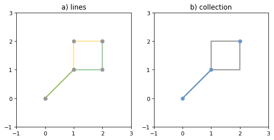
Figure 5. a) a green and a yellow line that intersect along a line and at a single point; b) the intersection (in blue) is a collection containing one LineString and one Point.
Members of a GeometryCollection are accessed via the geoms property.
>>> list(x.geoms)
[<LINESTRING (0 0, 1 1)>, <POINT (2 2)>]
Note
When possible, it is better to use one of the homogeneous collection types described below.
Collections of Points#
- class MultiPoint(points)#
The MultiPoint constructor takes a sequence of
(x, y[, z ])point tuples.
A MultiPoint has zero area and zero length.
>>> from shapely import MultiPoint
>>> points = MultiPoint([(0.0, 0.0), (1.0, 1.0)])
>>> points.area
0.0
>>> points.length
0.0
Its x-y bounding box is a (minx, miny, maxx, maxy) tuple.
>>> points.bounds
(0.0, 0.0, 1.0, 1.0)
Members of a multi-point collection are accessed via the geoms property.
>>> list(points.geoms)
[<POINT (0 0)>, <POINT (1 1)>]
The constructor also accepts another MultiPoint instance or an unordered sequence of Point instances, thereby making copies.
>>> MultiPoint([Point(0, 0), Point(1, 1)])
<MULTIPOINT ((0 0), (1 1))>
Collections of Lines#
- class MultiLineString(lines)#
The MultiLineString constructor takes a sequence of line-like sequences or objects.
(Source code, png, hires.png, pdf)

Figure 6. On the left, a simple, disconnected MultiLineString, and on the right, a non-simple MultiLineString. The points defining the objects are shown in gray, the boundaries of the objects in black.
A MultiLineString has zero area and non-zero length if it isn’t empty.
>>> from shapely import MultiLineString
>>> coords = [((0, 0), (1, 1)), ((-1, 0), (1, 0))]
>>> lines = MultiLineString(coords)
>>> lines.area
0.0
>>> lines.length
3.414213562373095
Its x-y bounding box is a (minx, miny, maxx, maxy) tuple.
>>> lines.bounds
(-1.0, 0.0, 1.0, 1.0)
Its members are instances of LineString and are accessed via the geoms
property.
>>> len(lines.geoms)
2
>>> print(list(lines.geoms))
[<LINESTRING (0 0, 1 1)>, <LINESTRING (-1 0, 1 0)>]
The constructor also accepts another instance of MultiLineString or an unordered sequence of LineString instances, thereby making copies.
>>> MultiLineString(lines)
<MULTILINESTRING ((0 0, 1 1), (-1 0, 1 0))>
>>> MultiLineString(lines.geoms)
<MULTILINESTRING ((0 0, 1 1), (-1 0, 1 0))>
Collections of Polygons#
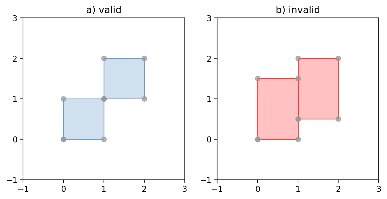
- class MultiPolygon(polygons)#
The MultiPolygon constructor takes a sequence of exterior ring and hole list tuples: [((a1, …, aM), [(b1, …, bN), …]), …].
More clearly, the constructor also accepts an unordered sequence of Polygon instances, thereby making copies.
>>> from shapely import MultiPolygon
>>> polygons = MultiPolygon([polygon, s, t])
>>> len(polygons.geoms)
3
(Source code, png, hires.png, pdf)
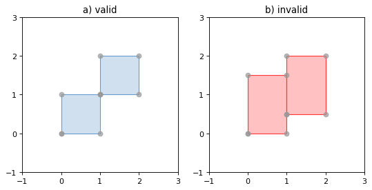
Figure 7. On the left, a valid MultiPolygon with 2 members, and on the right, a MultiPolygon that is invalid because its members touch at an infinite number of points (along a line).
Its x-y bounding box is a (minx, miny, maxx, maxy) tuple.
>>> polygons.bounds
(-1.0, -1.0, 2.0, 2.0)
Its members are instances of Polygon and are accessed via the geoms
property.
>>> len(polygons.geoms)
3
Empty features#
An “empty” feature is one with a point set that coincides with the empty set;
not None, but like set([]). Empty features can be created by calling
the various constructors with no arguments. Almost no operations are supported
by empty features.
>>> line = LineString()
>>> line.is_empty
True
>>> line.length
0.0
>>> line.bounds
(nan, nan, nan, nan)
>>> list(line.coords)
[]
Coordinate sequences#
The list of coordinates that describe a geometry are represented as the
CoordinateSequence object. These sequences should not be initialised
directly, but can be accessed from an existing geometry as the
Geometry.coords property.
>>> line = LineString([(0, 1), (2, 3), (4, 5)])
>>> line.coords
<shapely.coords.CoordinateSequence object at ...>
Coordinate sequences can be indexed, sliced and iterated over as if they were a list of coordinate tuples.
>>> line.coords[0]
(0.0, 1.0)
>>> line.coords[1:]
[(2.0, 3.0), (4.0, 5.0)]
>>> for x, y in line.coords:
...     print("x={}, y={}".format(x, y))
...
x=0.0, y=1.0
x=2.0, y=3.0
x=4.0, y=5.0
Polygons have a coordinate sequence for their exterior and each of their interior rings.
>>> poly = Polygon([(0, 0), (0, 1), (1, 1), (0, 0)])
>>> poly.exterior.coords
<shapely.coords.CoordinateSequence object at ...>
Multipart geometries do not have a coordinate sequence. Instead the coordinate sequences are stored on their component geometries.
>>> p = MultiPoint([(0, 0), (1, 1), (2, 2)])
>>> p.geoms[2].coords
<shapely.coords.CoordinateSequence object at ...>
Linear Referencing Methods#
It can be useful to specify position along linear features such as LineStrings and MultiLineStrings with a 1-dimensional referencing system. Shapely supports linear referencing based on length or distance, evaluating the distance along a geometric object to the projection of a given point, or the point at a given distance along the object.
- object.interpolate(distance[, normalized=False])#
Return a point at the specified distance along a linear geometric object.
If the normalized arg is True, the distance will be interpreted as a
fraction of the geometric object’s length.
>>> ip = LineString([(0, 0), (0, 1), (1, 1)]).interpolate(1.5)
>>> ip
<POINT (0.5 1)>
>>> LineString([(0, 0), (0, 1), (1, 1)]).interpolate(0.75, normalized=True)
<POINT (0.5 1)>
- object.project(other[, normalized=False])#
Returns the distance along this geometric object to a point nearest the other object.
If the normalized arg is True, return the distance normalized to the
length of the object. The project() method is the inverse of
interpolate().
>>> LineString([(0, 0), (0, 1), (1, 1)]).project(ip)
1.5
>>> LineString([(0, 0), (0, 1), (1, 1)]).project(ip, normalized=True)
0.75
For example, the linear referencing methods might be used to cut lines at a specified distance.
def cut(line, distance):
    # Cuts a line in two at a distance from its starting point
    if distance <= 0.0 or distance >= line.length:
        return [LineString(line)]
    coords = list(line.coords)
    for i, p in enumerate(coords):
        pd = line.project(Point(p))
        if pd == distance:
            return [
                LineString(coords[:i+1]),
                LineString(coords[i:])]
        if pd > distance:
            cp = line.interpolate(distance)
            return [
                LineString(coords[:i] + [(cp.x, cp.y)]),
                LineString([(cp.x, cp.y)] + coords[i:])]
>>> line = LineString([(0, 0), (1, 0), (2, 0), (3, 0), (4, 0), (5, 0)])
>>> print([list(x.coords) for x in cut(line, 1.0)])
[[(0.0, 0.0), (1.0, 0.0)],
 [(1.0, 0.0), (2.0, 0.0), (3.0, 0.0), (4.0, 0.0), (5.0, 0.0)]]
>>> print([list(x.coords) for x in cut(line, 2.5)])
[[(0.0, 0.0), (1.0, 0.0), (2.0, 0.0), (2.5, 0.0)],
 [(2.5, 0.0), (3.0, 0.0), (4.0, 0.0), (5.0, 0.0)]]
Predicates and Relationships#
Objects of the types explained in Geometric Objects provide standard [1]
predicates as attributes (for unary predicates) and methods (for binary
predicates). Whether unary or binary, all return True or False.
Unary Predicates#
Standard unary predicates are implemented as read-only property attributes. An example will be shown for each.
- object.has_z#
Returns
Trueif the feature has z coordinates, either with XYZ or XYZM coordinate types.
>>> Point(0, 0).has_z
False
>>> Point(0, 0, 0).has_z
True
- object.has_m#
Returns
Trueif the feature has m coordinates, either with XYM or XYZM coordinate types.New in version 2.1 with GEOS 3.12.
>>> Point(0, 0, 0).has_m
False
>>> from shapely import from_wkt
>>> from_wkt("POINT M (0 0 0)").has_m
True
- object.is_ccw#
Returns
Trueif coordinates are in counter-clockwise order (bounding a region with positive signed area). This method applies to LinearRing objects only.New in version 1.2.10.
>>> LinearRing([(1,0), (1,1), (0,0)]).is_ccw
True
A ring with an undesired orientation can be reversed like this:
>>> ring = LinearRing([(0,0), (1,1), (1,0)])
>>> ring.is_ccw
False
>>> ring2 = LinearRing(list(ring.coords)[::-1])
>>> ring2.is_ccw
True
- object.is_empty#
Returns
Trueif the feature’s interior and boundary (in point set terms) coincide with the empty set.
>>> Point().is_empty
True
>>> Point(0, 0).is_empty
False
Note
With the help of the operator module’s
attrgetter() function,
unary predicates such as is_empty can be easily used as predicates for
the built in filter().
>>> from operator import attrgetter
>>> empties = filter(attrgetter('is_empty'), [Point(), Point(0, 0)])
>>> len(list(empties))
1
- object.is_ring#
Returns
Trueif the feature is a closed and simpleLineString. A closed feature’s boundary coincides with the empty set.
>>> LineString([(0, 0), (1, 1), (1, -1)]).is_ring
False
>>> LinearRing([(0, 0), (1, 1), (1, -1)]).is_ring
True
This property is applicable to LineString and LinearRing instances, but meaningless for others.
- object.is_simple#
Returns
Trueif the feature does not cross itself.
Note
The simplicity test is meaningful only for LineStrings and LinearRings.
>>> LineString([(0, 0), (1, 1), (1, -1), (0, 1)]).is_simple
False
Operations on non-simple LineStrings are fully supported by Shapely.
A valid Polygon may not possess any overlapping exterior or interior rings. A valid MultiPolygon may not collect any overlapping polygons. A valid LineString must have non-zero length if it isn’t empty. Operations on invalid features may fail.
>>> MultiPolygon([Point(0, 0).buffer(2.0), Point(1, 1).buffer(2.0)]).is_valid
False
The two points above are close enough that the polygons resulting from the buffer operations (explained in a following section) overlap.
Note
The is_valid predicate can be used to write a validating decorator that
could ensure that only valid objects are returned from a constructor
function.
from functools import wraps
def validate(func):
    @wraps(func)
    def wrapper(*args, **kwargs):
        ob = func(*args, **kwargs)
        if not ob.is_valid:
            raise TopologicalError(
                "Given arguments do not determine a valid geometric object")
        return ob
    return wrapper
>>> @validate
... def ring(coordinates):
...     return LinearRing(coordinates)
...
>>> coords = [(0, 0), (1, 1), (1, -1), (0, 1)]
>>> ring(coords)
Traceback (most recent call last):
  File "<stdin>", line 1, in <module>
  File "<stdin>", line 7, in wrapper
shapely.geos.TopologicalError: Given arguments do not determine a valid geometric object
Binary Predicates#
Standard binary predicates are implemented as methods. These predicates
evaluate topological, set-theoretic relationships. In a few cases the results
may not be what one might expect starting from different assumptions. All take
another geometric object as argument and return True or False.
- object.__eq__(other)#
Returns
Trueif the two objects are of the same geometric type, and the coordinates of the two objects match precisely.
- object.equals(other)#
Returns
Trueif the set-theoretic boundary, interior, and exterior of the object coincide with those of the other.
The coordinates passed to the object constructors are of these sets, and determine them, but are not the entirety of the sets. This is a potential “gotcha” for new users. Equivalent lines, for example, can be constructed differently.
>>> a = LineString([(0, 0), (1, 1)])
>>> b = LineString([(0, 0), (0.5, 0.5), (1, 1)])
>>> c = LineString([(0, 0), (0, 0), (1, 1)])
>>> a.equals(b)
True
>>> a == b
False
>>> b.equals(c)
True
>>> b == c
False
- object.equals_exact(other, tolerance=0.0, normalize=False)#
Returns
Trueif the geometries are structurally equivalent within a given tolerance.This method uses exact coordinate equality, which requires coordinates to be equal (within specified tolerance) and in the same order for all components (vertices, rings, or parts) of a geometry. This is in contrast with the
equals()function which uses spatial (topological) equality and does not require all components to be in the same order. Because of this, it is possible forequals()to beTruewhileequals_exact()isFalse.The order of the coordinates can be normalized (by setting the normalize keyword to
True) so that this function will returnTruewhen geometries are structurally equivalent but differ only in the ordering of vertices. However, this function will still returnFalseif the order of interior rings within aPolygonor the order of geometries within a multi geometry are different.
>>> p1 = Point(1.0, 1.0)
>>> p2 = Point(2.0, 2.0)
>>> p3 = Point(1.0, 1.0 + 1e-7)
>>> p1.equals_exact(p2)
False
>>> p1.equals_exact(p3)
False
>>> p1.equals_exact(p3, tolerance=1e-6)
True
- object.contains(other)#
Returns
Trueif no points of other lie in the exterior of the object and at least one point of the interior of other lies in the interior of object.
This predicate applies to all types, and is inverse to within().
The expression a.contains(b) == b.within(a) always evaluates to True.
>>> coords = [(0, 0), (1, 1)]
>>> LineString(coords).contains(Point(0.5, 0.5))
True
>>> Point(0.5, 0.5).within(LineString(coords))
True
A line’s endpoints are part of its boundary and are therefore not contained.
>>> LineString(coords).contains(Point(1.0, 1.0))
False
Note
Binary predicates can be used directly as predicates for filter() or
itertools.ifilter().
>>> line = LineString(coords)
>>> contained = list(filter(line.contains, [Point(), Point(0.5, 0.5)]))
>>> len(contained)
1
>>> contained
[<POINT (0.5 0.5)>]
- object.covers(other)#
Returns
Trueif every point of other is a point on the interior or boundary of object. This is similar toobject.contains(other)except that this does not require any interior points of other to lie in the interior of object.
- object.covered_by(other)#
Returns
Trueif every point of object is a point on the interior or boundary of other. This is equivalent toother.covers(object).New in version 1.8.
- object.crosses(other)#
Returns
Trueif the interior of the object intersects the interior of the other but does not contain it, and the dimension of the intersection is less than the dimension of the one or the other.
>>> LineString(coords).crosses(LineString([(0, 1), (1, 0)]))
True
A line does not cross a point that it contains.
>>> LineString(coords).crosses(Point(0.5, 0.5))
False
- object.disjoint(other)#
Returns
Trueif the boundary and interior of the object do not intersect at all with those of the other.
>>> Point(0, 0).disjoint(Point(1, 1))
True
This predicate applies to all types and is the inverse of
intersects().
- object.intersects(other)#
Returns
Trueif the boundary or interior of the object intersect in any way with those of the other.
In other words, geometric objects intersect if they have any boundary or interior point in common.
- object.overlaps(other)#
Returns
Trueif the geometries have more than one but not all points in common, have the same dimension, and the intersection of the interiors of the geometries has the same dimension as the geometries themselves.
- object.touches(other)#
Returns
Trueif the objects have at least one point in common and their interiors do not intersect with any part of the other.
Overlapping features do not therefore touch, another potential “gotcha”. For
example, the following lines touch at (1, 1), but do not overlap.
>>> a = LineString([(0, 0), (1, 1)])
>>> b = LineString([(1, 1), (2, 2)])
>>> a.touches(b)
True
- object.within(other)#
Return
Trueif the object is completely inside the other.
This applies to all types and is the inverse of contains().
For more details on the exact behaviour, check out shapely.within().
Used in a sorted() key, within() makes it easy to spatially
sort objects. Let’s say we have 4 stereotypic features: a point that is
contained by a polygon which is itself contained by another polygon, and a free
spirited point contained by none
>>> a = Point(2, 2)
>>> b = Polygon([[1, 1], [1, 3], [3, 3], [3, 1]])
>>> c = Polygon([[0, 0], [0, 4], [4, 4], [4, 0]])
>>> d = Point(-1, -1)
and that copies of these are collected into a list
>>> features = [c, a, d, b, c]
that we’d prefer to have ordered as [d, c, c, b, a] in reverse containment
order.
DE-9IM Relationships#
The relate() method tests all the DE-9IM [4] relationships
between objects, of which the named relationship predicates above are a subset.
- object.relate(other)#
Returns a string representation of the DE-9IM matrix of relationships between an object’s interior, boundary, exterior and those of another geometric object.
The named relationship predicates (contains(), etc.) are
typically implemented as wrappers around relate().
Two different points have mainly F (false) values in their matrix; the
intersection of their external sets (the 9th element) is a 2 dimensional
object (the rest of the plane). The intersection of the interior of one with
the exterior of the other is a 0 dimensional object (3rd and 7th elements
of the matrix).
>>> Point(0, 0).relate(Point(1, 1))
'FF0FFF0F2'
The matrix for a line and a point on the line has more “true” (not F)
elements.
>>> Point(0, 0).relate(LineString([(0, 0), (1, 1)]))
'F0FFFF102'
- object.relate_pattern(other, pattern)#
Returns True if the DE-9IM string code for the relationship between the geometries satisfies the pattern, otherwise False.
The relate_pattern() compares the DE-9IM code string for two
geometries against a specified pattern. If the string matches the pattern then
True is returned, otherwise False. The pattern specified can be an
exact match (0, 1 or 2), a boolean match (T or F), or a
wildcard (*). For example, the pattern for the within predicate is
T*****FF*.
>>> point = Point(0.5, 0.5)
>>> square = Polygon([(0, 0), (0, 1), (1, 1), (1, 0)])
>>> square.relate_pattern(point, 'T*****FF*')
True
>>> point.within(square)
True
Note that the order or the geometries is significant, as demonstrated below. In this example the square contains the point, but the point does not contain the square.
>>> point.relate(square)
'0FFFFF212'
>>> square.relate(point)
'0F2FF1FF2'
Further discussion of the DE-9IM matrix is beyond the scope of this manual. See [4] and https://pypi.org/project/de9im/.
Spatial Analysis Methods#
As well as boolean attributes and methods, Shapely provides analysis methods that return new geometric objects.
Set-theoretic Methods#
Almost every binary predicate method has a counterpart that returns a new geometric object. In addition, the set-theoretic boundary of an object is available as a read-only attribute.
Note
These methods will always return a geometric object. An intersection of
disjoint geometries for example will return an empty GeometryCollection,
not None or False. To test for a non-empty result, use the geometry’s
is_empty property.
- object.boundary#
Returns a lower dimensional object representing the object’s set-theoretic boundary.
The boundary of a polygon is a line, the boundary of a line is a collection of points. The boundary of a point is an empty collection.
>>> coords = [((0, 0), (1, 1)), ((-1, 0), (1, 0))]
>>> lines = MultiLineString(coords)
>>> lines.boundary
<MULTIPOINT ((-1 0), (0 0), (1 0), (1 1))>
>>> list(lines.boundary.geoms)
[<POINT (-1 0)>, <POINT (0 0)>, <POINT (1 0)>, <POINT (1 1)>]
>>> lines.boundary.boundary
<GEOMETRYCOLLECTION EMPTY>
See the figures in LineStrings and Collections of Lines for the illustration of lines and their boundaries.
- object.centroid#
Returns a representation of the object’s geometric centroid (point).
>>> LineString([(0, 0), (1, 1)]).centroid
<POINT (0.5 0.5)>
Note
The centroid of an object might be one of its points, but this is not guaranteed.
- object.difference(other)#
Returns a representation of the points making up this geometric object that do not make up the other object.
>>> a = Point(1, 1).buffer(1.5)
>>> b = Point(2, 1).buffer(1.5)
>>> a.difference(b)
<POLYGON ((1.435 -0.435, 1.293 -0.471, 1.147 -0.493, 1 -0.5, 0.853 -0.493, 0...>
Note
The buffer() method is used to produce approximately circular polygons
in the examples of this section; it will be explained in detail later in this
manual.
(Source code, png, hires.png, pdf)
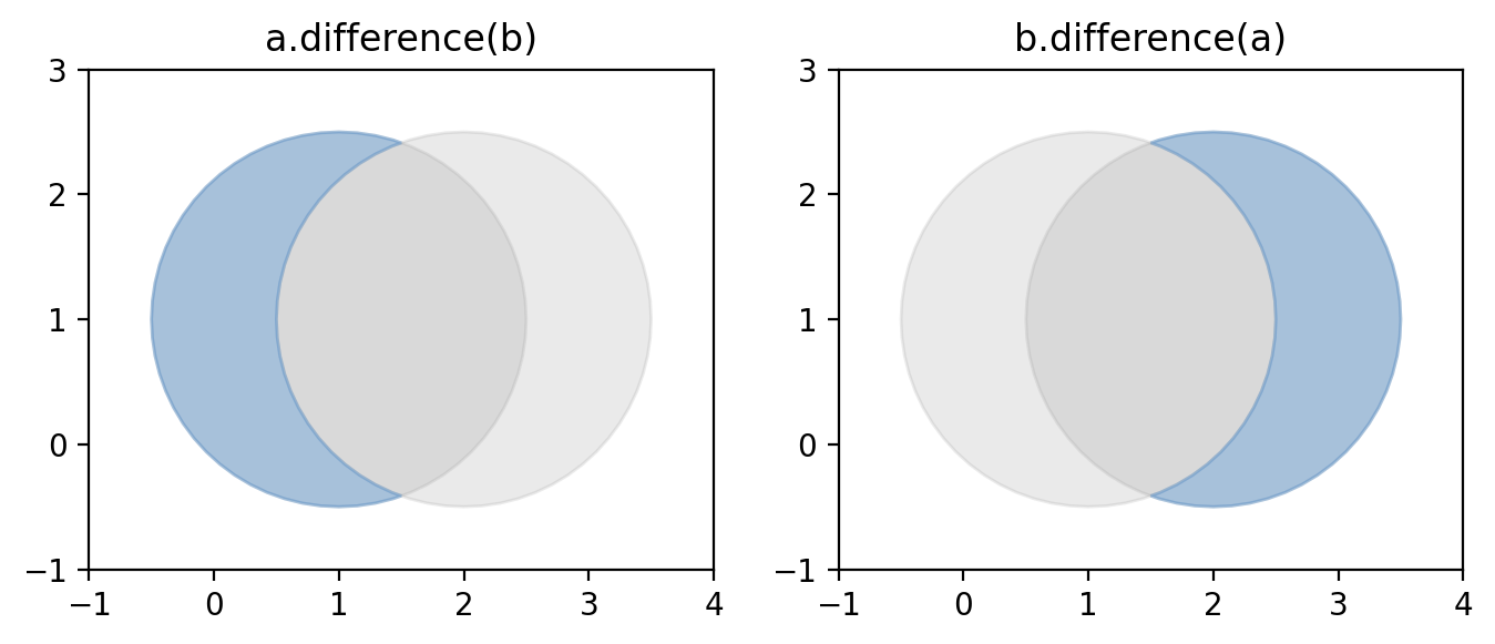
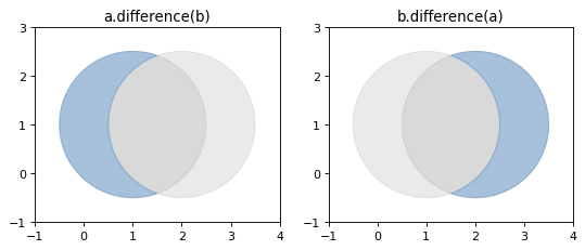
Figure 8. Differences between two approximately circular polygons.
Note
Shapely can not represent the difference between an object and a lower
dimensional object (such as the difference between a polygon and a line or
point) as a single object, and in these cases the difference method returns a
deep copy of the object named self.
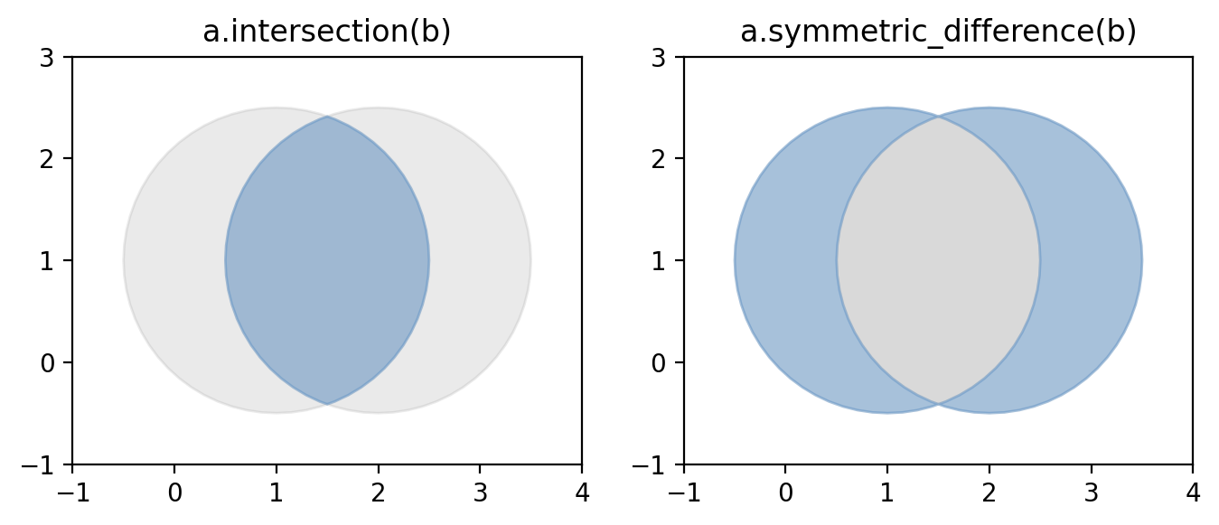
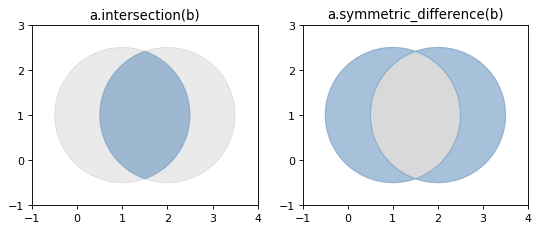
- object.intersection(other)#
Returns a representation of the intersection of this object with the other geometric object.
>>> a = Point(1, 1).buffer(1.5)
>>> b = Point(2, 1).buffer(1.5)
>>> a.intersection(b)
<POLYGON ((2.493 0.853, 2.471 0.707, 2.435 0.565, 2.386 0.426, 2.323 0.293, ...>
See the figure under symmetric_difference() below.
- object.symmetric_difference(other)#
Returns a representation of the points in this object not in the other geometric object, and the points in the other not in this geometric object.
>>> a = Point(1, 1).buffer(1.5)
>>> b = Point(2, 1).buffer(1.5)
>>> a.symmetric_difference(b)
<MULTIPOLYGON (((1.574 -0.386, 1.707 -0.323, 1.833 -0.247, 1.952 -0.16, 2.06...>
(Source code, png, hires.png, pdf)
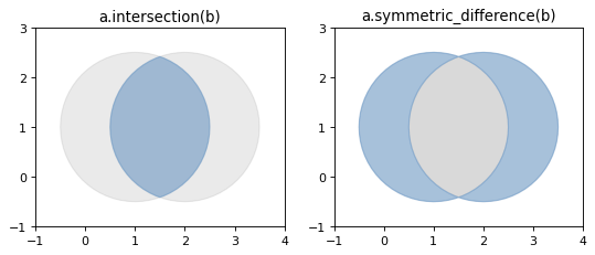
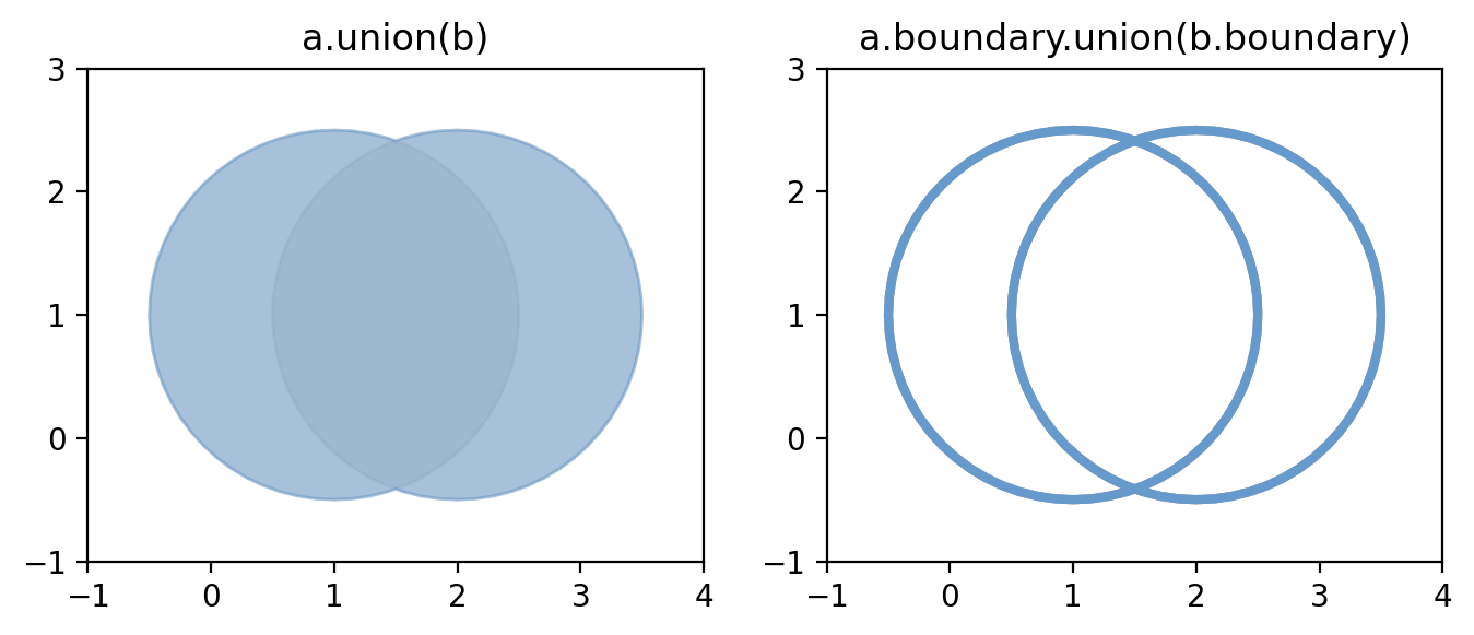
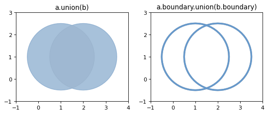
- object.union(other)#
Returns a representation of the union of points from this object and the other geometric object.
The type of object returned depends on the relationship between the operands. The union of polygons (for example) will be a polygon or a multi-polygon depending on whether they intersect or not.
>>> a = Point(1, 1).buffer(1.5)
>>> b = Point(2, 1).buffer(1.5)
>>> a.union(b)
<POLYGON ((1.435 -0.435, 1.293 -0.471, 1.147 -0.493, 1 -0.5, 0.853 -0.493, 0...>
The semantics of these operations vary with type of geometric object. For example, compare the boundary of the union of polygons to the union of their boundaries.
>>> a.union(b).boundary
<LINESTRING (1.435 -0.435, 1.293 -0.471, 1.147 -0.493, 1 -0.5, 0.853 -0.493,...>
>>> a.boundary.union(b.boundary)
<MULTILINESTRING ((2.5 1, 2.493 0.853, 2.471 0.707, 2.435 0.565, 2.386 0.426...>
(Source code, png, hires.png, pdf)
Note
union() is an expensive way to find the cumulative union
of many objects. See shapely.unary_union() for a more effective
method.
Several of these set-theoretic methods can be invoked using overloaded operators:
intersection can be accessed with and, &
union can be accessed with or, |
difference can be accessed with minus, -
symmetric_difference can be accessed with xor, ^
>>> from shapely import wkt
>>> p1 = wkt.loads('POLYGON((0 0, 1 0, 1 1, 0 1, 0 0))')
>>> p2 = wkt.loads('POLYGON((0.5 0, 1.5 0, 1.5 1, 0.5 1, 0.5 0))')
>>> p1 & p2
<POLYGON ((0.5 0, 0.5 1, 1 1, 1 0, 0.5 0))>
>>> p1 | p2
<POLYGON ((0 0, 0 1, 0.5 1, 1 1, 1.5 1, 1.5 0, 1 0, 0.5 0, 0 0))>
>>> p1 - p2
<POLYGON ((0 0, 0 1, 0.5 1, 0.5 0, 0 0))>
>>> (p1 ^ p2).wkt
'MULTIPOLYGON (((0 0, 0 1, 0.5 1, 0.5 0, 0 0)), ((1 1, 1.5 1, 1.5 0, 1 0, 1 1)))'
Constructive Methods#
Shapely geometric object have several methods that yield new objects not derived from set-theoretic analysis.
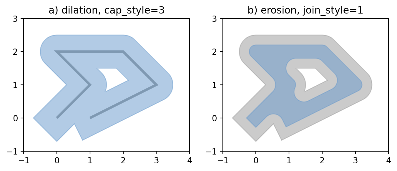
- object.buffer(distance, quad_segs=16, cap_style=1, join_style=1, mitre_limit=5.0, single_sided=False)#
Returns an approximate representation of all points within a given distance of the this geometric object.
The styles of caps are specified by integer values: 1 (round), 2 (flat), 3 (square). These values are also enumerated by the object
shapely.BufferCapStyle(see below).The styles of joins between offset segments are specified by integer values: 1 (round), 2 (mitre), and 3 (bevel). These values are also enumerated by the object
shapely.BufferJoinStyle(see below).
- shapely.BufferCapStyle#
Attribute
Value
round
1
flat
2
square
3
- shapely.BufferJoinStyle#
Attribute
Value
round
1
mitre
2
bevel
3
>>> from shapely import BufferCapStyle, BufferJoinStyle
>>> BufferCapStyle.flat.value
2
>>> BufferJoinStyle.bevel.value
3
A positive distance has an effect of dilation; a negative distance, erosion. The optional quad_segs argument determines the number of segments used to approximate a quarter circle around a point.
>>> line = LineString([(0, 0), (1, 1), (0, 2), (2, 2), (3, 1), (1, 0)])
>>> dilated = line.buffer(0.5)
>>> eroded = dilated.buffer(-0.3)
(Source code, png, hires.png, pdf)
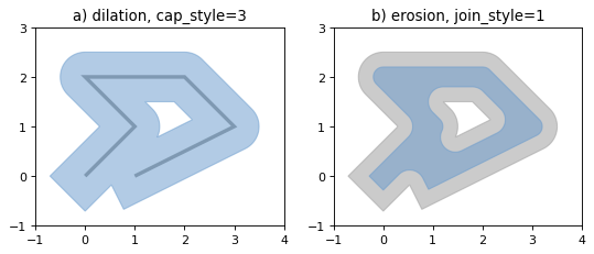
Figure 9. Dilation of a line (left) and erosion of a polygon (right). New object is shown in blue.
The default (quad_segs of 16) buffer of a point is a polygonal patch with 99.8% of the area of the circular disk it approximates.
>>> p = Point(0, 0).buffer(10.0)
>>> len(p.exterior.coords)
65
>>> p.area
313.6548490545941
With a quad_segs of 1, the buffer is a square patch.
>>> q = Point(0, 0).buffer(10.0, 1)
>>> len(q.exterior.coords)
5
>>> q.area
200.0
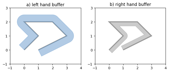
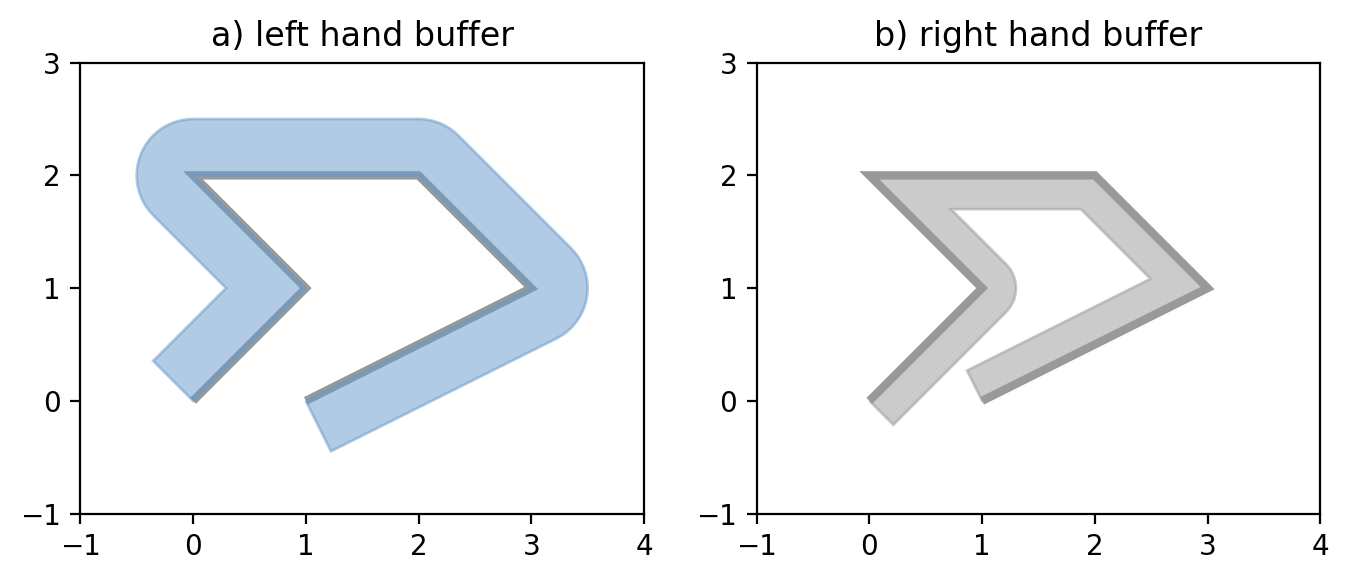
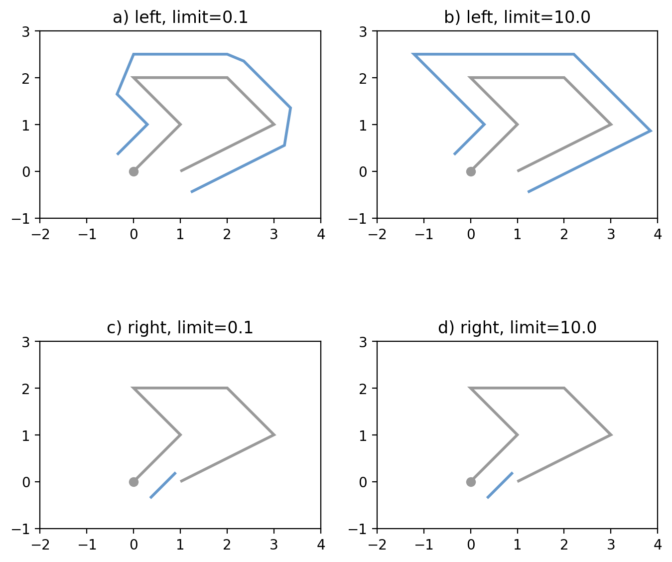
You may want a buffer only on one side. You can achieve this effect with single_sided option.
The side used is determined by the sign of the buffer distance:
a positive distance indicates the left-hand side
a negative distance indicates the right-hand side
>>> line = LineString([(0, 0), (1, 1), (0, 2), (2, 2), (3, 1), (1, 0)])
>>> left_hand_side = line.buffer(0.5, single_sided=True)
>>> right_hand_side = line.buffer(-0.3, single_sided=True)
(Source code, png, hires.png, pdf)

Figure 10. Single sided buffer of 0.5 left hand (left) and of 0.3 right hand (right).
The single-sided buffer of point geometries is the same as the regular buffer. The End Cap Style for single-sided buffers is always ignored, and forced to the equivalent of BufferCapStyle.flat.
Passed a distance of 0, buffer() can sometimes be used to
“clean” self-touching or self-crossing polygons such as the classic “bowtie”.
Users have reported that very small distance values sometimes produce cleaner
results than 0. Your mileage may vary when cleaning surfaces.
>>> coords = [(0, 0), (0, 2), (1, 1), (2, 2), (2, 0), (1, 1), (0, 0)]
>>> bowtie = Polygon(coords)
>>> bowtie.is_valid
False
>>> clean = bowtie.buffer(0)
>>> clean.is_valid
True
>>> clean
<MULTIPOLYGON (((0 0, 0 2, 1 1, 0 0)), ((1 1, 2 2, 2 0, 1 1)))>
>>> len(clean.geoms)
2
>>> list(clean.geoms[0].exterior.coords)
[(0.0, 0.0), (0.0, 2.0), (1.0, 1.0), (0.0, 0.0)]
>>> list(clean.geoms[1].exterior.coords)
[(1.0, 1.0), (2.0, 2.0), (2.0, 0.0), (1.0, 1.0)]
Buffering splits the polygon in two at the point where they touch.
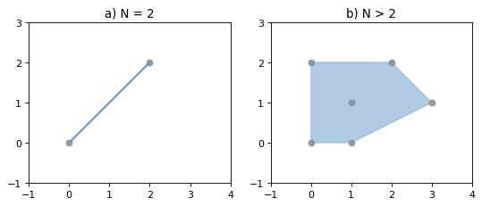
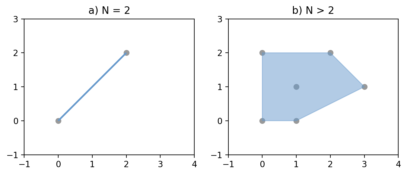
- object.convex_hull#
Returns a representation of the smallest convex Polygon containing all the points in the object unless the number of points in the object is less than three. For two points, the convex hull collapses to a LineString; for 1, a Point.
>>> Point(0, 0).convex_hull
<POINT (0 0)>
>>> MultiPoint([(0, 0), (1, 1)]).convex_hull
<LINESTRING (0 0, 1 1)>
>>> MultiPoint([(0, 0), (1, 1), (1, -1)]).convex_hull
<POLYGON ((1 -1, 0 0, 1 1, 1 -1))>
(Source code, png, hires.png, pdf)

Figure 11. Convex hull (blue) of 2 points (left) and of 6 points (right).
- object.envelope#
Returns a representation of the point or smallest rectangular polygon (with sides parallel to the coordinate axes) that contains the object.
>>> Point(0, 0).envelope
<POINT (0 0)>
>>> MultiPoint([(0, 0), (1, 1)]).envelope
<POLYGON ((0 0, 1 0, 1 1, 0 1, 0 0))>
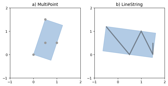
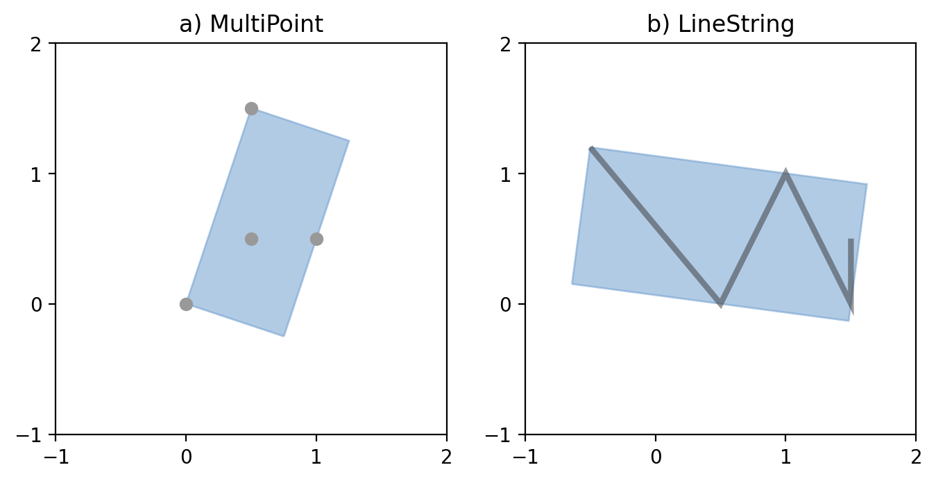
- object.minimum_rotated_rectangle#
Returns the general minimum bounding rectangle that contains the object. Unlike envelope this rectangle is not constrained to be parallel to the coordinate axes. If the convex hull of the object is a degenerate (line or point) this degenerate is returned.
New in Shapely 1.6.0
>>> Point(0, 0).minimum_rotated_rectangle
<POINT (0 0)>
>>> MultiPoint([(0,0),(1,1),(2,0.5)]).minimum_rotated_rectangle.normalize()
<POLYGON ((-0.176 0.706, 1.824 1.206, 2 0.5, 0 0, -0.176 0.706))>
(Source code, png, hires.png, pdf)

Figure 12. Minimum rotated rectangle for a multipoint feature (left) and a linestring feature (right).
- object.parallel_offset(distance, side, resolution=16, join_style=1, mitre_limit=5.0)#
Returns a LineString or MultiLineString geometry at a distance from the object on its right or its left side.
Older alternative method to the
offset_curve()method, but uses resolution instead of quad_segs and a side keyword (‘left’ or ‘right’) instead of sign of the distance. This method is kept for backwards compatibility for now, but is is recommended to useoffset_curve()instead.
- object.offset_curve(distance, quad_segs=16, join_style=1, mitre_limit=5.0)#
Returns a LineString or MultiLineString geometry at a distance from the object on its right or its left side.
The distance parameter must be a float value.
The side is determined by the sign of the distance parameter (negative for right side offset, positive for left side offset). Left and right are determined by following the direction of the given geometric points of the LineString.
Note: the behaviour regarding orientation of the resulting line depends on the GEOS version. With GEOS < 3.11, the line retains the same direction for a left offset (positive distance) or has reverse direction for a right offset (negative distance), and this behaviour was documented as such in previous Shapely versions. Starting with GEOS 3.11, the function tries to preserve the orientation of the original line.
The resolution of the offset around each vertex of the object is parameterized as in the
buffer()method (using quad_segs).The join_style is for outside corners between line segments. Accepted integer values are 1 (round), 2 (mitre), and 3 (bevel). See also
shapely.BufferJoinStyle.Severely mitered corners can be controlled by the mitre_limit parameter (spelled in British English, en-gb). The corners of a parallel line will be further from the original than most places with the mitre join style. The ratio of this further distance to the specified distance is the miter ratio. Corners with a ratio which exceed the limit will be beveled.
Note
This method may sometimes return a MultiLineString where a simple LineString was expected; for example, an offset to a slightly curved LineString.
Note
This method is only available for LinearRing and LineString objects.
(Source code, png, hires.png, pdf)
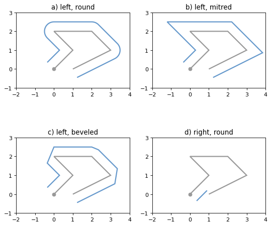
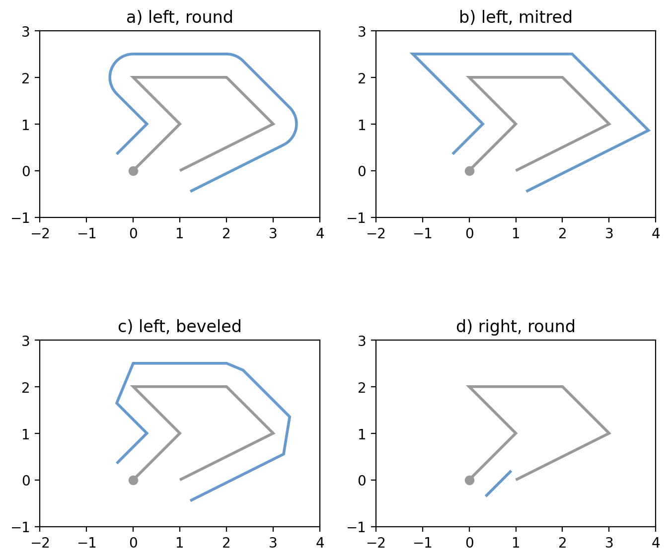
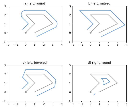
Figure 13. Three styles of parallel offset lines on the left side of a simple line string (its starting point shown as a circle) and one offset on the right side, a multipart.
The effect of the mitre_limit parameter is shown below.
(Source code, png, hires.png, pdf)
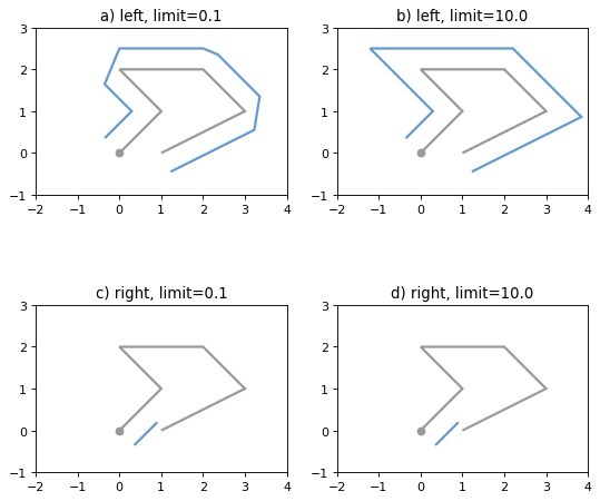
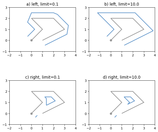
Figure 14. Large and small mitre_limit values for left and right offsets.
- object.simplify(tolerance, preserve_topology=True)#
Returns a simplified representation of the geometric object.
All points in the simplified object will be within the tolerance distance of
the original geometry. By default a slower algorithm is used that preserves
topology. If preserve topology is set to False the much quicker
Douglas-Peucker algorithm [6] is used.
>>> p = Point(0.0, 0.0)
>>> x = p.buffer(1.0)
>>> x.area
3.1365484905459398
>>> len(x.exterior.coords)
65
>>> s = x.simplify(0.05, preserve_topology=False)
>>> s.area
3.061467458920719
>>> len(s.exterior.coords)
17
(Source code, png, hires.png, pdf)
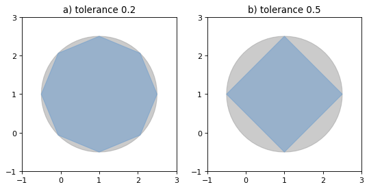
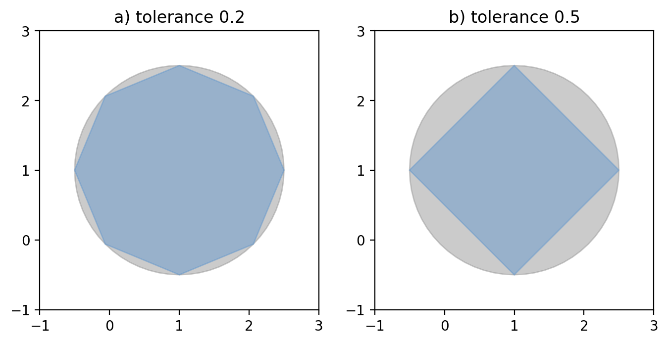

Figure 15. Simplification of a nearly circular polygon using a tolerance of 0.2 (left) and 0.5 (right).
Note
Invalid geometric objects may result from simplification that does not preserve topology and simplification may be sensitive to the order of coordinates: two geometries differing only in order of coordinates may be simplified differently.
Affine Transformations#
A collection of affine transform functions are in the shapely.affinity
module, which return transformed geometries by either directly supplying
coefficients to an affine transformation matrix, or by using a specific, named
transform (rotate, scale, etc.). The functions can be used with all
geometry types (except GeometryCollection), and 3D types are either
preserved or supported by 3D affine transformations.
New in version 1.2.17.
- shapely.affinity.affine_transform(geom, matrix)#
Returns a transformed geometry using an affine transformation matrix.
The coefficient
matrixis provided as a list or tuple with 6 or 12 items for 2D or 3D transformations, respectively.For 2D affine transformations, the 6 parameter
matrixis:[a, b, d, e, xoff, yoff]which represents the augmented matrix:
\[\begin{split}\begin{bmatrix} x' \\ y' \\ 1 \end{bmatrix} = \begin{bmatrix} a & b & x_\mathrm{off} \\ d & e & y_\mathrm{off} \\ 0 & 0 & 1 \end{bmatrix} \begin{bmatrix} x \\ y \\ 1 \end{bmatrix}\end{split}\]or the equations for the transformed coordinates:
\[\begin{split}x' &= a x + b y + x_\mathrm{off} \\ y' &= d x + e y + y_\mathrm{off}.\end{split}\]For 3D affine transformations, the 12 parameter
matrixis:[a, b, c, d, e, f, g, h, i, xoff, yoff, zoff]which represents the augmented matrix:
\[\begin{split}\begin{bmatrix} x' \\ y' \\ z' \\ 1 \end{bmatrix} = \begin{bmatrix} a & b & c & x_\mathrm{off} \\ d & e & f & y_\mathrm{off} \\ g & h & i & z_\mathrm{off} \\ 0 & 0 & 0 & 1 \end{bmatrix} \begin{bmatrix} x \\ y \\ z \\ 1 \end{bmatrix}\end{split}\]or the equations for the transformed coordinates:
\[\begin{split}x' &= a x + b y + c z + x_\mathrm{off} \\ y' &= d x + e y + f z + y_\mathrm{off} \\ z' &= g x + h y + i z + z_\mathrm{off}.\end{split}\]
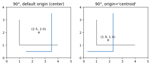
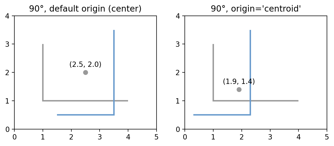
- shapely.affinity.rotate(geom, angle, origin='center', use_radians=False)#
Returns a rotated geometry on a 2D plane.
The angle of rotation can be specified in either degrees (default) or radians by setting
use_radians=True. Positive angles are counter-clockwise and negative are clockwise rotations.The point of origin can be a keyword
'center'for the bounding box center (default),'centroid'for the geometry’s centroid, a Point object or a coordinate tuple(x0, y0).The affine transformation matrix for 2D rotation with angle \(\theta\) is:
\[\begin{split}\begin{bmatrix} \cos{\theta} & -\sin{\theta} & x_\mathrm{off} \\ \sin{\theta} & \cos{\theta} & y_\mathrm{off} \\ 0 & 0 & 1 \end{bmatrix}\end{split}\]where the offsets are calculated from the origin \((x_0, y_0)\):
\[\begin{split}x_\mathrm{off} &= x_0 - x_0 \cos{\theta} + y_0 \sin{\theta} \\ y_\mathrm{off} &= y_0 - x_0 \sin{\theta} - y_0 \cos{\theta}\end{split}\]>>> from shapely import affinity >>> line = LineString([(1, 3), (1, 1), (4, 1)]) >>> rotated_a = affinity.rotate(line, 90) >>> rotated_b = affinity.rotate(line, 90, origin='centroid')
(
Source code,png,hires.png,pdf)
Figure 16. Rotation of a LineString (gray) by an angle of 90° counter-clockwise (blue) using different origins.
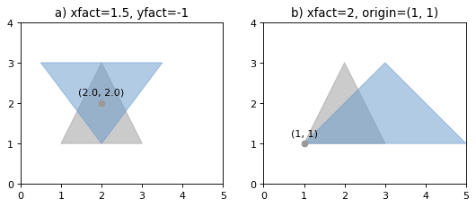
- shapely.affinity.scale(geom, xfact=1.0, yfact=1.0, zfact=1.0, origin='center')#
Returns a scaled geometry, scaled by factors along each dimension.
The point of origin can be a keyword
'center'for the 2D bounding box center (default),'centroid'for the geometry’s 2D centroid, a Point object or a coordinate tuple(x0, y0, z0).Negative scale factors will mirror or reflect coordinates.
The general 3D affine transformation matrix for scaling is:
\[\begin{split}\begin{bmatrix} x_\mathrm{fact} & 0 & 0 & x_\mathrm{off} \\ 0 & y_\mathrm{fact} & 0 & y_\mathrm{off} \\ 0 & 0 & z_\mathrm{fact} & z_\mathrm{off} \\ 0 & 0 & 0 & 1 \end{bmatrix}\end{split}\]where the offsets are calculated from the origin \((x_0, y_0, z_0)\):
\[\begin{split}x_\mathrm{off} &= x_0 - x_0 x_\mathrm{fact} \\ y_\mathrm{off} &= y_0 - y_0 y_\mathrm{fact} \\ z_\mathrm{off} &= z_0 - z_0 z_\mathrm{fact}\end{split}\]>>> triangle = Polygon([(1, 1), (2, 3), (3, 1)]) >>> triangle_a = affinity.scale(triangle, xfact=1.5, yfact=-1) >>> triangle_a.exterior.coords[:] [(0.5, 3.0), (2.0, 1.0), (3.5, 3.0), (0.5, 3.0)] >>> triangle_b = affinity.scale(triangle, xfact=2, origin=(1,1)) >>> triangle_b.exterior.coords[:] [(1.0, 1.0), (3.0, 3.0), (5.0, 1.0), (1.0, 1.0)]
(
Source code,png,hires.png,pdf)
Figure 17. Scaling of a gray triangle to blue result: a) by a factor of 1.5 along x-direction, with reflection across y-axis; b) by a factor of 2 along x-direction with custom origin at (1, 1).
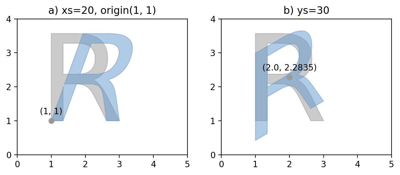
- shapely.affinity.skew(geom, xs=0.0, ys=0.0, origin='center', use_radians=False)#
Returns a skewed geometry, sheared by angles along x and y dimensions.
The shear angle can be specified in either degrees (default) or radians by setting
use_radians=True.The point of origin can be a keyword
'center'for the bounding box center (default),'centroid'for the geometry’s centroid, a Point object or a coordinate tuple(x0, y0).The general 2D affine transformation matrix for skewing is:
\[\begin{split}\begin{bmatrix} 1 & \tan{x_s} & x_\mathrm{off} \\ \tan{y_s} & 1 & y_\mathrm{off} \\ 0 & 0 & 1 \end{bmatrix}\end{split}\]where the offsets are calculated from the origin \((x_0, y_0)\):
\[\begin{split}x_\mathrm{off} &= -y_0 \tan{x_s} \\ y_\mathrm{off} &= -x_0 \tan{y_s}\end{split}\](
Source code,png,hires.png,pdf)
Figure 18. Skewing of a gray “R” to blue result: a) by a shear angle of 20° along the x-direction and an origin at (1, 1); b) by a shear angle of 30° along the y-direction, using default origin.
- shapely.affinity.translate(geom, xoff=0.0, yoff=0.0, zoff=0.0)#
Returns a translated geometry shifted by offsets along each dimension.
The general 3D affine transformation matrix for translation is:
\[\begin{split}\begin{bmatrix} 1 & 0 & 0 & x_\mathrm{off} \\ 0 & 1 & 0 & y_\mathrm{off} \\ 0 & 0 & 1 & z_\mathrm{off} \\ 0 & 0 & 0 & 1 \end{bmatrix}\end{split}\]
Other Transformations#
Shapely supports map projections and other arbitrary transformations of geometric objects.
- shapely.ops.transform(func, geom)#
Applies func to all coordinates of geom and returns a new geometry of the same type from the transformed coordinates.
func maps x, y, and optionally z to output xp, yp, zp. The input parameters may be iterable types like lists or arrays or single values. The output shall be of the same type: scalars in, scalars out; lists in, lists out.
transform tries to determine which kind of function was passed in by calling func first with n iterables of coordinates, where n is the dimensionality of the input geometry. If func raises a TypeError when called with iterables as arguments, then it will instead call func on each individual coordinate in the geometry.
New in version 1.2.18.
For example, here is an identity function applicable to both types of input (scalar or array).
def id_func(x, y, z=None):
    return tuple(filter(None, [x, y, z]))

g2 = transform(id_func, g1)
If using pyproj>=2.1.0, the preferred method to project geometries is:
import pyproj

from shapely import Point
from shapely.ops import transform

wgs84_pt = Point(-72.2495, 43.886)

wgs84 = pyproj.CRS('EPSG:4326')
utm = pyproj.CRS('EPSG:32618')

project = pyproj.Transformer.from_crs(wgs84, utm, always_xy=True).transform
utm_point = transform(project, wgs84_pt)
It is important to note that in the example above, the always_xy kwarg is required as Shapely only supports coordinates in X,Y order, and in PROJ 6 the WGS84 CRS uses the EPSG-defined Lat/Lon coordinate order instead of the expected Lon/Lat.
If using pyproj < 2.1, then the canonical example is:
from functools import partial
import pyproj

from shapely.ops import transform

wgs84 = pyproj.Proj(init='epsg:4326')
utm = pyproj.Proj(init='epsg:32618')

project = partial(
    pyproj.transform,
    wgs84,
    utm)

utm_point = transform(project, wgs84_pt)
Lambda expressions such as the one in
g2 = transform(lambda x, y, z=None: (x+1.0, y+1.0), g1)
also satisfy the requirements for func.
Other Operations#
Merging Linear Features#
Sequences of touching lines can be merged into MultiLineStrings or Polygons.
- shapely.polygonize(lines)#
Returns an iterator over polygons constructed from the input lines.
The source should be a sequence of LineString objects.
>>> from shapely import polygonize
>>> lines = [
...     LineString([(0, 0), (1, 1)]),
...     LineString([(0, 0), (0, 1)]),
...     LineString([(0, 1), (1, 1)]),
...     LineString([(1, 1), (1, 0)]),
...     LineString([(1, 0), (0, 0)]),
...     ]
>>> list(polygonize(lines).geoms)
[<POLYGON ((0 0, 1 1, 1 0, 0 0))>, <POLYGON ((1 1, 0 0, 0 1, 1 1))>]
- shapely.polygonize_full(lines)#
Creates polygons from a source of lines, returning the polygons and leftover geometries.
The source should be a sequence of LineString objects.
Returns a tuple of objects: (polygons, cut edges, dangles, invalid ring lines). Each are a geometry collection.
Dangles are edges which have one or both ends which are not incident on another edge endpoint. Cut edges are connected at both ends but do not form part of polygon. Invalid ring lines form rings which are invalid (bowties, etc).
New in version 1.2.18.
>>> from shapely import polygonize_full
>>> lines = [
...     LineString([(0, 0), (1, 1)]),
...     LineString([(0, 0), (0, 1)]),
...     LineString([(0, 1), (1, 1)]),
...     LineString([(1, 1), (1, 0)]),
...     LineString([(1, 0), (0, 0)]),
...     LineString([(5, 5), (6, 6)]),
...     LineString([(1, 1), (100, 100)]),
...     ]
>>> result, cuts, dangles, invalids = polygonize_full(lines)
>>> len(result.geoms)
2
>>> list(result.geoms)
[<POLYGON ((0 0, 1 1, 1 0, 0 0))>, <POLYGON ((1 1, 0 0, 0 1, 1 1))>]
>>> list(dangles.geoms)
[<LINESTRING (1 1, 100 100)>, <LINESTRING (5 5, 6 6)>]
- shapely.line_merge(multilinestring)#
Returns LineString(s) or MultiLineString(s) representing the merger of all contiguous elements of the input MultiLineString(s).
>>> from shapely import line_merge
>>> line_merge(MultiLineString(lines))
<MULTILINESTRING ((1 1, 1 0, 0 0), (0 0, 1 1), (0 0, 0 1, 1 1), (1 1, 100 10...>
>>> list(line_merge(MultiLineString(lines)).geoms)
[<LINESTRING (1 1, 1 0, 0 0)>,
 <LINESTRING (0 0, 1 1)>,
 <LINESTRING (0 0, 0 1, 1 1)>,
 <LINESTRING (1 1, 100 100)>,
 <LINESTRING (5 5, 6 6)>]
Efficient Rectangle Clipping#
The clip_by_rect() function returns the portion of a geometry
within a rectangle.
- shapely.clip_by_rect(geom, xmin, ymin, xmax, ymax)#
The geometry is clipped in a fast but possibly dirty way. The output is not guaranteed to be valid. No exceptions will be raised for topological errors.
New in version 1.7.
>>> from shapely import clip_by_rect
>>> polygon = Polygon(
...     shell=[(0, 0), (0, 30), (30, 30), (30, 0), (0, 0)],
...     holes=[[(10, 10), (20, 10), (20, 20), (10, 20), (10, 10)]],
... )
>>> clipped_polygon = clip_by_rect(polygon, 5, 5, 15, 15)
>>> clipped_polygon
<POLYGON ((5 5, 5 15, 10 15, 10 10, 15 10, 15 5, 5 5))>
Efficient Unions#
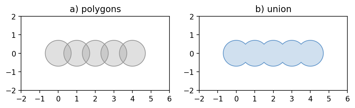
The unary_union() function is more efficient than accumulating
with union().
(Source code, png, hires.png, pdf)
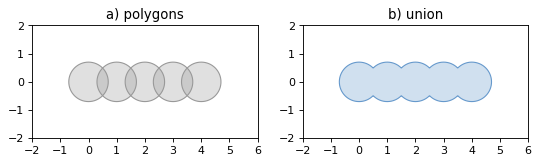
- shapely.unary_union(geoms)#
Returns a representation of the union of the given geometric objects.
Areas of overlapping Polygons will get merged. LineStrings will get fully dissolved and noded. Duplicate Points will get merged.
>>> from shapely import unary_union
>>> polygons = [Point(i, 0).buffer(0.7) for i in range(5)]
>>> unary_union(polygons)
<POLYGON ((0.444 -0.541, 0.389 -0.582, 0.33 -0.617, 0.268 -0.647, 0.203 -0.6...>
Because the union merges the areas of overlapping Polygons it can be used in an attempt to fix invalid MultiPolygons. As with the zero distance
buffer()trick, your mileage may vary when using this.>>> m = MultiPolygon(polygons) >>> m.area 7.684543801837549 >>> m.is_valid False >>> unary_union(m).area 6.610301355116799 >>> unary_union(m).is_valid True
Delaunay triangulation#
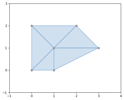
The delaunay_triangles() function calculates a Delaunay
triangulation from a collection of points.
(Source code, png, hires.png, pdf)

- shapely.delaunay_triangles(geom, tolerance=0.0, edges=False)#
Returns a Delaunay triangulation of the vertices of the input geometry.
The source may be any geometry type. All vertices of the geometry will be used as the points of the triangulation.
The tolerance keyword argument sets the snapping tolerance used to improve the robustness of the triangulation computation. A tolerance of 0.0 specifies that no snapping will take place.
If the edges keyword argument is False a list of Polygon triangles will be returned. Otherwise a list of LineString edges is returned.
New in version 1.4.0
>>> from shapely import delaunay_triangles
>>> points = MultiPoint([(0, 0), (1, 1), (0, 2), (2, 2), (3, 1), (1, 0)])
>>> list(delaunay_triangles(points).geoms)
[<POLYGON ((0 2, 0 0, 1 1, 0 2))>,
 <POLYGON ((0 2, 1 1, 2 2, 0 2))>,
 <POLYGON ((2 2, 1 1, 3 1, 2 2))>,
 <POLYGON ((3 1, 1 1, 1 0, 3 1))>,
 <POLYGON ((1 0, 1 1, 0 0, 1 0))>]
Voronoi Diagram#
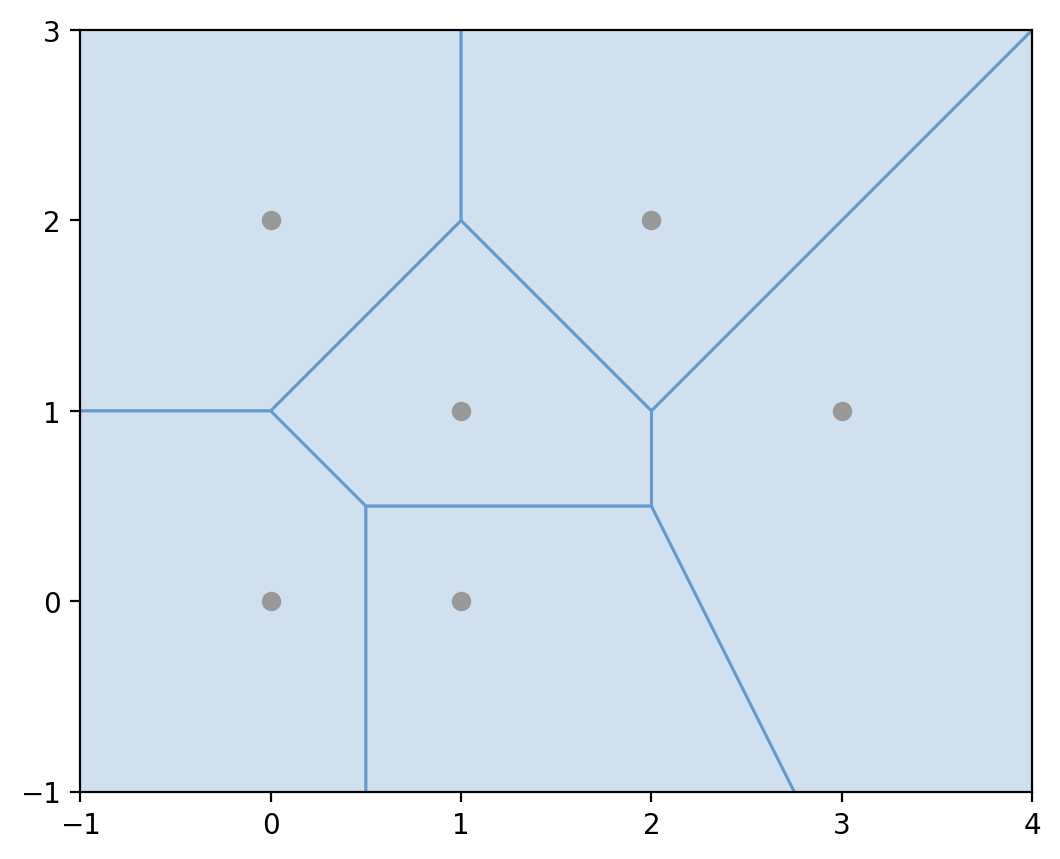
The voronoi_polygons() function constructs a Voronoi diagram
from a collection points, or the vertices of any geometry.
(Source code, png, hires.png, pdf)
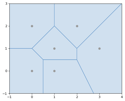
- shapely.voronoi_polygons(geom, envelope=None, tolerance=0.0, edges=False)#
Constructs a Voronoi diagram from the vertices of the input geometry.
The source may be any geometry type. All vertices of the geometry will be used as the input points to the diagram.
The envelope keyword argument provides an envelope to use to clip the resulting diagram. If None, it will be calculated automatically. The diagram will be clipped to the larger of the provided envelope or an envelope surrounding the sites.
The tolerance keyword argument sets the snapping tolerance used to improve the robustness of the computation. A tolerance of 0.0 specifies that no snapping will take place. The tolerance argument can be finicky and is known to cause the algorithm to fail in several cases. If you’re using tolerance and getting a failure, try removing it. The test cases in tests/test_voronoi_diagram.py show more details.
If the edges keyword argument is False a list of Polygon`s will be returned. Otherwise a list of `LineString edges is returned.
>>> from shapely import voronoi_polygons
>>> points = MultiPoint([(0, 0), (1, 1), (0, 2), (2, 2), (3, 1), (1, 0)])
>>> regions = voronoi_polygons(points)
>>> list(regions.geoms)
[<POLYGON ((2 1, 2 0.5, 0.5 0.5, 0 1, 1 2, 2 1))>,
 <POLYGON ((6 -3, 3.75 -3, 2 0.5, 2 1, 6 5, 6 -3))>,
 <POLYGON ((-3 -3, -3 1, 0 1, 0.5 0.5, 0.5 -3, -3 -3))>,
 <POLYGON ((0.5 -3, 0.5 0.5, 2 0.5, 3.75 -3, 0.5 -3))>,
 <POLYGON ((-3 5, 1 5, 1 2, 0 1, -3 1, -3 5))>,
 <POLYGON ((6 5, 2 1, 1 2, 1 5, 6 5))>]
Nearest points/shortest line#
The shortest_line() function calculates the shortest line
between a pair of geometries.
- shapely.shortest_line(geom1, geom2)#
Returns a tuple of the shortest line between the input geometries. The points are returned in the same order as the input geometries.
New in version 2.0.
>>> from shapely import shortest_line
>>> triangle = Polygon([(0, 0), (1, 0), (0.5, 1), (0, 0)])
>>> square = Polygon([(0, 2), (1, 2), (1, 3), (0, 3), (0, 2)])
>>> shortest_line(triangle, square)
<LINESTRING (0.5 1, 0.5 2)>
Note that the shortest line may not connect to vertices of the input geometries.
Snapping#
The snap() snaps the vertices in one geometry to the vertices in
a second geometry with a given tolerance.
- shapely.snap(geom1, geom2, tolerance)#
Snaps vertices in geom1 to vertices in the geom2. A new instance of type geom1 is returned. The input geometries are not modified.
The tolerance argument specifies the minimum distance between vertices for them to be snapped.
New in version 1.5.0
>>> from shapely import snap
>>> square = Polygon([(1,1), (2, 1), (2, 2), (1, 2), (1, 1)])
>>> line = LineString([(0,0), (0.8, 0.8), (1.8, 0.95), (2.6, 0.5)])
>>> result = snap(line, square, 0.5)
>>> result
<LINESTRING (0 0, 1 1, 2 1, 2.6 0.5)>
Splitting#
The split() function in shapely.ops splits a geometry by
another geometry.
- shapely.ops.split(geom, splitter)#
Splits a geometry by another geometry and returns a collection of geometries. This function is the theoretical opposite of the union of the split geometry parts. If the splitter does not split the geometry, a collection with a single geometry equal to the input geometry is returned.
The function supports:
Splitting a (Multi)LineString by a (Multi)Point or (Multi)LineString or (Multi)Polygon boundary
Splitting a (Multi)Polygon by a LineString
It may be convenient to snap the splitter with low tolerance to the geometry. For example in the case of splitting a line by a point, the point must be exactly on the line, for the line to be correctly split. When splitting a line by a polygon, the boundary of the polygon is used for the operation. When splitting a line by another line, a ValueError is raised if the two overlap at some segment.
>>> from shapely.ops import split
>>> pt = Point((1, 1))
>>> line = LineString([(0,0), (2,2)])
>>> result = split(line, pt)
>>> result
<GEOMETRYCOLLECTION (LINESTRING (0 0, 1 1), LINESTRING (1 1, 2 2))>
Substring#
The substring() function in shapely.ops returns a
line segment between specified distances along a LineString.
- shapely.ops.substring(geom, start_dist, end_dist[, normalized=False])#
Return the LineString between start_dist and end_dist or a Point if they are at the same location
Negative distance values are taken as measured in the reverse direction from the end of the geometry. Out-of-range index values are handled by clamping them to the valid range of values.
If the start distance equals the end distance, a point is being returned.
If the start distance is actually past the end distance, then the reversed substring is returned such that the start distance is at the first coordinate.
If the normalized arg is
True, the distance will be interpreted as a fraction of the geometry’s lengthNew in version 1.7.0
Here are some examples that return LineString geometries.
>>> from shapely.ops import substring
>>> ls = LineString((i, 0) for i in range(6))
>>> ls
<LINESTRING (0 0, 1 0, 2 0, 3 0, 4 0, 5 0)>
>>> substring(ls, start_dist=1, end_dist=3)
<LINESTRING (1 0, 2 0, 3 0)>
>>> substring(ls, start_dist=3, end_dist=1)
<LINESTRING (3 0, 2 0, 1 0)>
>>> substring(ls, start_dist=1, end_dist=-3)
<LINESTRING (1 0, 2 0)>
>>> substring(ls, start_dist=0.2, end_dist=-0.6, normalized=True)
<LINESTRING (1 0, 2 0)>
And here is an example that returns a Point.
>>> substring(ls, start_dist=2.5, end_dist=-2.5)
<POINT (2.5 0)>
Prepared Geometry Operations#
Shapely geometries can be processed into a state that supports more efficient batches of operations.
- prepared.prep(ob)#
Creates and returns a prepared geometric object.
To test one polygon containment against a large batch of points, one should
first use the prepared.prep() function.
>>> from shapely.prepared import prep
>>> points = [...] # large list of points
>>> polygon = Point(0.0, 0.0).buffer(1.0)
>>> prepared_polygon = prep(polygon)
>>> prepared_polygon
<shapely.prepared.PreparedGeometry object at 0x...>
>>> hits = filter(prepared_polygon.contains, points)
You can use the same Binary Predicates on prepared geometries as on normal geometries. All have exactly the same arguments and usage as their counterparts in non-prepared geometric objects, but execution will be faster.
Diagnostics#
- validation.explain_validity(ob):
Returns a string explaining the validity or invalidity of the object.
New in version 1.2.1.
The messages may or may not have a representation of a problem point that can be parsed out.
>>> coords = [(0, 0), (0, 2), (1, 1), (2, 2), (2, 0), (1, 1), (0, 0)]
>>> p = Polygon(coords)
>>> from shapely.validation import explain_validity
>>> explain_validity(p)
'Ring Self-intersection[1 1]'
- validation.make_valid(ob)#
Returns a valid representation of the geometry, if it is invalid. If it is valid, the input geometry will be returned.
In many cases, in order to create a valid geometry, the input geometry must be split into multiple parts or multiple geometries. If the geometry must be split into multiple parts of the same geometry type, then a multi-part geometry (e.g. a MultiPolygon) will be returned. if the geometry must be split into multiple parts of different types, then a GeometryCollection will be returned.
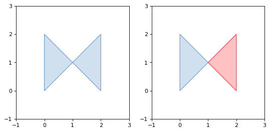
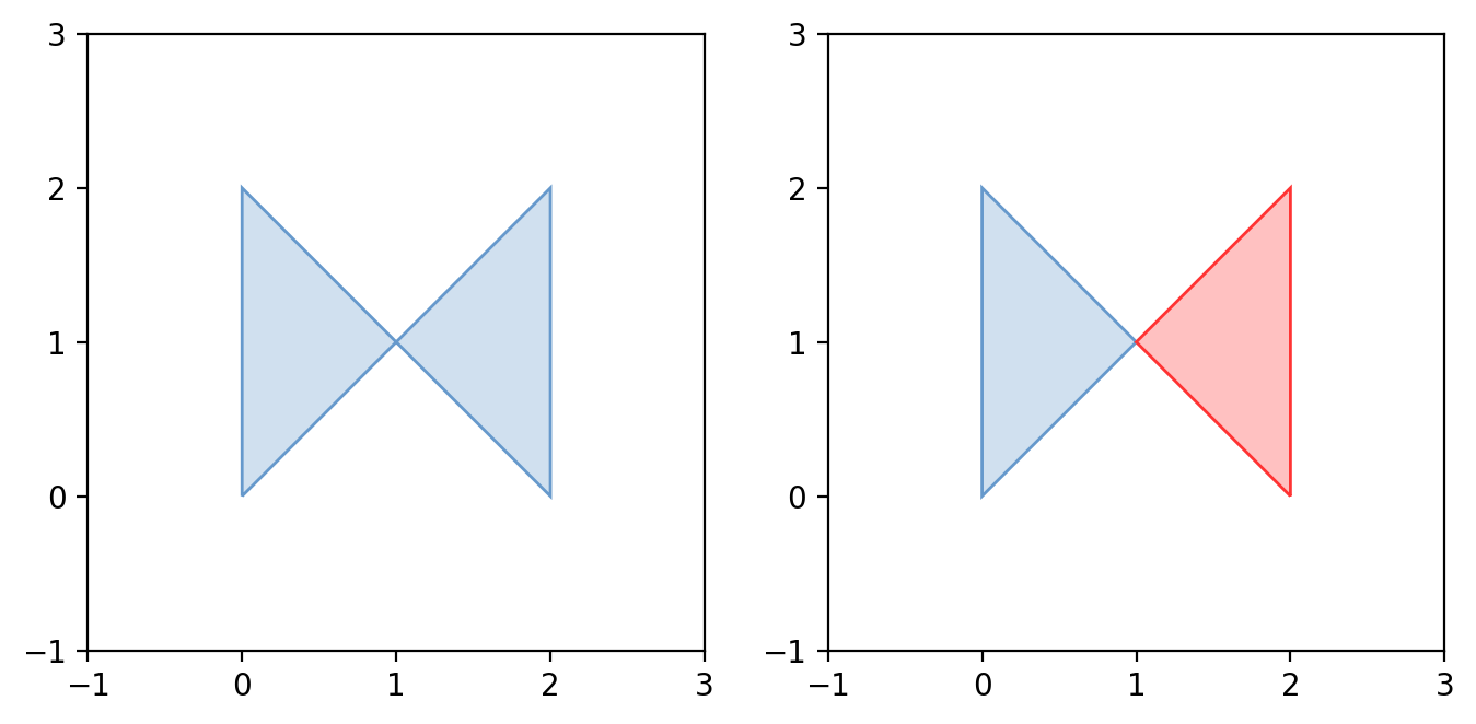
For example, this operation on a geometry with a bow-tie structure:
>>> from shapely.validation import make_valid
>>> coords = [(0, 0), (0, 2), (1, 1), (2, 2), (2, 0), (1, 1), (0, 0)]
>>> p = Polygon(coords)
>>> make_valid(p)
<MULTIPOLYGON (((1 1, 0 0, 0 2, 1 1)), ((2 0, 1 1, 2 2, 2 0)))>

Yields a MultiPolygon with two parts:
(Source code, png, hires.png, pdf)

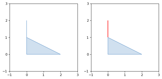
While this operation:#
>>> from shapely.validation import make_valid
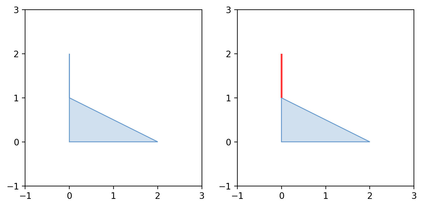
>>> coords = [(0, 2), (0, 1), (2, 0), (0, 0), (0, 2)]
>>> p = Polygon(coords)
>>> make_valid(p)
<GEOMETRYCOLLECTION (POLYGON ((2 0, 0 0, 0 1, 2 0)), LINESTRING (0 2, 0 1))>
Yields a GeometryCollection with a Polygon and a LineString:
(Source code, png, hires.png, pdf)

New in version 1.8#
The Shapely version, GEOS library version, and GEOS C API version are
accessible via shapely.__version__, shapely.geos_version_string, and
shapely.geos_capi_version.
>>> import shapely
>>> shapely.__version__
'2.0.0'
>>> shapely.geos_version
(3, 10, 2)
>>> shapely.geos_capi_version_string
'3.10.2-CAPI-1.16.0'
Polylabel#
- shapely.ops.polylabel(polygon, tolerance)#
Finds the approximate location of the pole of inaccessibility for a given polygon. Based on Vladimir Agafonkin’s polylabel.
New in version 1.6.0
Note
Prior to 1.7 polylabel must be imported from shapely.algorithms.polylabel instead of shapely.ops.
>>> from shapely.ops import polylabel
>>> polygon = LineString([(0, 0), (50, 200), (100, 100), (20, 50),
... (-100, -20), (-150, -200)]).buffer(100)
>>> label = polylabel(polygon, tolerance=0.001)
>>> label
<POINT (59.733 111.33)>
STR-packed R-tree#
Shapely provides an interface to the query-only GEOS R-tree packed using the Sort-Tile-Recursive algorithm. Pass a list of geometry objects to the STRtree constructor to create a spatial index that you can query with another geometric object. Query-only means that once created, the STRtree is immutable. You cannot add or remove geometries.
- class strtree.STRtree(geometries)
The STRtree constructor takes a sequence of geometric objects.
References to these geometric objects are kept and stored in the R-tree.
New in version 1.4.0.
- strtree.query(geom)
Returns the integer indices of all geometries in the strtree whose extents intersect the extent of geom. This means that a subsequent search through the returned subset using the desired binary predicate (eg. intersects, crosses, contains, overlaps) may be necessary to further filter the results according to their specific spatial relationships.
>>> from shapely import STRtree
>>> points = [Point(i, i) for i in range(10)]
>>> tree = STRtree(points)
>>> query_geom = Point(2,2).buffer(0.99)
>>> [points[idx].wkt for idx in tree.query(query_geom)]
['POINT (2 2)']
>>> query_geom = Point(2, 2).buffer(1.0)
>>> [points[idx].wkt for idx in tree.query(query_geom)]
['POINT (1 1)', 'POINT (2 2)', 'POINT (3 3)']
>>> [points[idx].wkt for idx in tree.query(query_geom, predicate="intersects")]
['POINT (2 2)']
- strtree.nearest(geom)
Returns the nearest geometry in strtree to geom.
>>> points = [Point(i, i) for i in range(10)]
>>> tree = STRtree(points)
>>> idx = tree.nearest(Point(2.2, 2.2))
>>> points[idx]
<POINT (2 2)>
Interoperation#
Shapely provides 4 avenues for interoperation with other software.
Well-Known Formats#
A Well Known Text (WKT) or Well Known Binary (WKB) representation [1] of
any geometric object can be had via its wkt or wkb attribute.
These representations allow interchange with many GIS programs. PostGIS, for
example, trades in hex-encoded WKB.
>>> Point(0, 0).wkt
'POINT (0 0)'
>>> Point(0, 0).wkb
b'\x01\x01\x00\x00\x00\x00\x00\x00\x00\x00\x00\x00\x00\x00\x00\x00\x00\x00\x00\x00\x00'
>>> Point(0, 0).wkb_hex
'010100000000000000000000000000000000000000'
The shapely.wkt and shapely.wkb modules provide dumps() and loads()
functions that work almost exactly as their pickle and simplejson module
counterparts. To serialize a geometric object to a binary or text string, use
dumps(). To deserialize a string and get a new geometric object of the
appropriate type, use loads().
The default settings for the wkt attribute and shapely.wkt.dumps() function are different. By default, the attribute’s value is trimmed of excess decimals, while this is not the case for dumps(), though it can be replicated by setting trim=True.
- shapely.wkb.dumps(ob)#
Returns a WKB representation of ob.
- shapely.wkb.loads(wkb)#
Returns a geometric object from a WKB representation wkb.
>>> from shapely import wkb, Point
>>> pt = Point(0, 0)
>>> wkb.dumps(pt)
b'\x01\x01\x00\x00\x00\x00\x00\x00\x00\x00\x00\x00\x00\x00\x00\x00\x00\x00\x00\x00\x00'
>>> pt.wkb
b'\x01\x01\x00\x00\x00\x00\x00\x00\x00\x00\x00\x00\x00\x00\x00\x00\x00\x00\x00\x00\x00'
>>> wkb.loads(pt.wkb).wkt
'POINT (0 0)'
All of Shapely’s geometry types are supported by these functions.
- shapely.wkt.dumps(ob)#
Returns a WKT representation of ob. Several keyword arguments are available to alter the WKT which is returned; see the docstrings for more details.
- shapely.wkt.loads(wkt)#
Returns a geometric object from a WKT representation wkt.
>>> from shapely import wkt, Point
>>> pt = Point(0, 0)
>>> wkt.dumps(pt)
'POINT (0.0000000000000000 0.0000000000000000)'
>>> pt.wkt
'POINT (0 0)'
>>> wkt.loads(pt.wkt).wkt
'POINT (0 0)'
Numpy and Python Arrays#
All geometric objects with coordinate sequences (Point, LinearRing, LineString) provide the Numpy array interface and can thereby be converted or adapted to Numpy arrays.
>>> import numpy as np
>>> np.asarray(Point(0, 0).coords)
array([[0., 0.]])
>>> np.asarray(LineString([(0, 0), (1, 1)]).coords)
array([[0., 0.],
       [1., 1.]])
The coordinates of the same types of geometric objects can be had as standard
Python arrays of x and y values via the xy attribute.
>>> Point(0, 0).xy
(array('d', [0.0]), array('d', [0.0]))
>>> LineString([(0, 0), (1, 1)]).xy
(array('d', [0.0, 1.0]), array('d', [0.0, 1.0]))
Python Geo Interface#
Any object that provides the GeoJSON-like Python geo interface can be
converted to a Shapely geometry using the shapely.geometry.shape()
function.
- shapely.geometry.shape(context)#
Returns a new, independent geometry with coordinates copied from the context.
For example, a dictionary:
>>> from shapely.geometry import shape
>>> data = {"type": "Point", "coordinates": (0.0, 0.0)}
>>> geom = shape(data)
>>> geom.geom_type
'Point'
>>> list(geom.coords)
[(0.0, 0.0)]
Or a simple placemark-type object:
>>> class GeoThing:
...     def __init__(self, d):
...         self.__geo_interface__ = d
>>> thing = GeoThing({"type": "Point", "coordinates": (0.0, 0.0)})
>>> geom = shape(thing)
>>> geom.geom_type
'Point'
>>> list(geom.coords)
[(0.0, 0.0)]
The GeoJSON-like mapping of a geometric object can be obtained using
shapely.geometry.mapping().
- shapely.geometry.mapping(ob)#
Returns a GeoJSON-like mapping from a Geometry or any object which implements
__geo_interface__.Note that
mappingdoes not enforce the winding order of polygons to be compliant with the RFC 7946 GeoJSON specification. If you want this, you can first order exterior rings counterclockwise, and interior rings (holes) clockwise withshapely.orient_polygons().New in version 1.2.3.
For example, using the same GeoThing class:
>>> from shapely.geometry import mapping
>>> thing = GeoThing({"type": "Point", "coordinates": (0.0, 0.0)})
>>> m = mapping(thing)
>>> m['type']
'Point'
>>> m['coordinates']
(0.0, 0.0)
Performance#
Shapely uses the GEOS library for all operations. GEOS is written in C++ and used in many applications and you can expect that all operations are highly optimized. The creation of new geometries with many coordinates, however, involves some overhead that might slow down your code.
Conclusion#
We hope that you will enjoy and profit from using Shapely. This manual will be updated and improved regularly. Its source is available at shapely/shapely.